16 Creating automatic analysis pipelines
Note🧑🏫 Instructor note
Before beginning, get them to recall what they remember of the previous session, either with something like Mentimeter, verbally, or using hands / stickies / origami hats. Preferably something that will allow everyone to participate, not just the ones who are more comfortable being vocal to the whole group.
Depending on what they write, you may need to briefly go over the previous session.
When doing analyses on data, you have probably experienced (many) times where you forget the order in which other code should run or which parts need to be rerun to update results. Things can get confusing quickly, even in relatively simple projects. This becomes even more challenging when you return to a project after a month or two and have forgotten the state of the analysis and the project as a whole.
That’s where formal data analysis pipeline tools come in. By organising your analysis into distinct steps, with clear inputs and outputs, and adding these steps to a pipeline that tracks them, you can make things a lot easier for yourself and others. This session focuses on using tools that create and manage these pipelines effectively.
16.1 Learning objectives
This session’s overall learning outcome is to:
- Apply an approach to build an analysis pipeline that clearly defines each step of your analysis—from raw data to finished manuscript— so that updates by you and your collaborators are as simple as running a single function.
More specific objectives are to:
- Describe the computational meaning of pipeline and how pipelines are often used in research. Explain why a well-designed pipeline can streamline collaboration, reduce time spent on an analysis, make the analysis steps explicit and easier to work with, and ultimately contribute to more fully reproducible research.
- Explain the difference between a “function-oriented” workflow and a “script-oriented” workflow, and why the function-based approach has multiple advantages from a time- and effort-efficiency point of view.
- Use the functions within targets to apply the concepts of building pipelines in your analysis project.
- Continue applying the concepts and functions introduced in the previous session
16.2 💬 Discussion activity: How do you rerun analyses when something changes?
Time: ~12 minutes.
We’ve all been in situations where something in our analysis needs to change: Maybe we forgot to remove a certain condition (like unrealistic BMI), maybe our supervisor suggests something we hadn’t considered in our analysis, or maybe during peer review of our manuscript, a reviewer makes a suggestion that would improve the understanding of the paper.
Whatever the situation, we inevitably need to rerun parts of or the full analysis. So what is your exact workflow when you need to rerun code and update your results? Assume it’s a change somewhere early in the data processing stage.
- Take about 1 minute to think about the workflow you use. Try to think of the exact steps you need to take, what exactly you do, and how long that usually takes.
- For 8 minutes, share and discuss your thoughts in your group. How do your experiences compare to each other?
- For the remaining time, we’ll briefly share with everyone what they’ve thought and discussed.
16.3 What is a data analysis “pipeline”?
Note🧑🏫 Instructor note
After they finish reading this section, briefly walk through it. In particular, emphasize what we want to make at the end, even though that goal might change as the analysis progresses.
Note📖 Reading task: ~10 minutes
A pipeline can be any process where the steps between a start and an end point are very clear, explicit, and concrete. These highly distinct steps can be manual, human involved, or completely automated by a robot or computer. For instance, in car factories, the pipeline from the input raw materials to the output vehicle is extremely well described and implemented. Similarly, during the pandemic, the pipeline for testing (at least in Denmark and several other countries) was highly structured and clear for both the workers doing the testing and the people having the test done: A person goes in, scans their ID card, has the test done, the worker inputs the results, and the results are sent immediately to the health agency as well as to the person based on their ID contact information (or via a secure app).
However, in research, especially around data collection and analysis, we often hear or read about “pipelines”. But looking closer, these aren’t actual pipelines because the individual steps are not very clear and not well described, and they often require a fair amount of manual human attention and intervention. Particularly within computational environments, a pipeline should be a set of data processing steps connected in a series with a specific order; the output of one step is the input to the next. This means that there actually should be minimal to no human intervention from raw input to finished output.
Why aren’t these computational data pipelines found in most of the “pipelines” described in research? Because:
- Anything with data ultimately must be on the computer,
- Anything automatically done on the computer must be done with code,
- Not all researchers write code,
- Researchers who do write code rarely publish and share it,
- Code that is shared or published (either publicly or within the research group) is not written in a way that allows a pipeline to exist,
- And, research is largely non-reproducible (1–3).
A data analysis pipeline would, by definition, be a readable and reproducible data analysis. Unfortunately, we researchers, as a group, don’t make use of the tools to implement actual data analysis pipelines.
This isn’t to diminish the work of researchers, but is rather a basic observation on the systemic, social, and structural environment surrounding us. We as researchers are not necessarily trained in writing code, nor do we have a strong culture and incentive structure around learning, sharing, reviewing, and improving code. We are also very rarely allowed to get (or use) funds to hire people who are trained and skilled in programmatic thinking and coding. Otherwise workshops like this wouldn’t need to exist 🤷♀️
Before we get to what an actual data analysis pipeline looks like in practice, we have to separate two things: exploratory data analysis and final paper data analysis. In exploratory data analysis, there will likely be a lot of manual, interactive steps involved that may or may not need to be explicitly stated and included in the analysis plan and pipeline. But for the final paper and the included results, we generally have some basic first ideas of what we’ll need. Let’s list a few items that we would want to do before the primary statistical analysis:
- A table of some basic descriptive statistics of the study population, such as mean, standard deviation, or counts of basic discrete data (like treatment group).
- A figure showing the distribution of your main variables of interest. In this case, ours are the lipidomic variables.
- The paper with the results included.
Now that we have conceptually drawn out some initial tasks in our pipeline, we can start using R to build it.
1.
Trisovic A, Lau MK, Pasquier T, Crosas M. A large-scale study on research code quality and execution. Scientific Data. 2022 Feb;9(1).
16.4 Using targets to manage a pipeline
There are a few packages that help build pipelines in R, but the most commonly used, well-designed, and maintained one is called targets. This package allows you to explicitly specify the outputs you want to create. targets will then track them for you and know which output depends on which as well as which ones need to be updated when you make changes to your pipeline.
Note🧑🏫 Instructor note
Ask participants, which do they think it is: a build dependency or a workflow dependency. Because it is directly used to run analyses and process the data, it would be a build dependency.
First, we need to install and add targets to our dependencies. Since targets is a build dependency, we’ll add it to the DESCRIPTION file with:
Console
use_package("targets")Now that it’s added to the project R library, let’s set up our project to start using it!
Console
targets::use_targets()This command will write a _targets.R script file that we’ll use to define our analysis pipeline. Before we do that though, let’s commit the file to the Git history with Ctrl-Alt-MCtrl-Alt-M or with the Palette (Ctrl-Shift-PCtrl-Shift-P, then type “commit”).
Note
If you are using an older version of the targets package, you might also find that running targets::use_targets() also have created a run.R and run.sh file. The files are used for other situations (like running on a Linux server) that we won’t cover in this workshop.
Note🧑🏫 Instructor note
Let them read it before going over it again to reinforce function-oriented workflows and how targets and the tar_target() works.
Note📖 Reading task: ~8
For this reading task, we’ll take a look at what the _targets.R contains. So, start by opening it on your computer.
Mostly, the_targets.R script contains comments and a basic set up to get you started. But, notice the tar_target() function used at the end of the script. There are two main arguments for it: name and command. The way that targets works is similar to how you’d assign the output of a function to an object, so:
object_name <- function_in_command(input_arguments)Is the same as:
tar_target(
  name = object_name,
  command = function_in_command(input_arguments)
)
What this means is that targets follows a “function-oriented” workflow, not a “script-based” workflow. What’s the difference? In a script-oriented workflow, each R file/script is run in a specific order. As a result, you might end up with an R file that has code like:
While in a function-oriented workflow, it might look more like:
source("R/functions.R")
raw_data <- load_raw_data("file/path/data.csv")
processed_data <- process_data(raw_data)
basic_stats <- calculate_basic_statistics(processed_data)
simple_plot <- create_plot(processed_data)
model_results <- run_linear_reg(processed_data)
With the function-oriented workflow, each function takes an input and contains all the code to create one result as its output. This could be, for instance, a figure in a paper.
If you’ve taken the intermediate R workshop, you’ll notice that this function-oriented workflow is the workflow we covered in that workshop. There are so many advantages to this type of workflow which is why many powerful R packages are designed around making use of this workflow.
If we take these same code as above and convert it into the targets format, the end of _targets.R file would like this:
list(
  tar_target(
    name = raw_data,
    command = load_raw_data("file/path/data.csv")
  ),
  tar_target(
    name = processed_data,
    command = process_data(raw_data)
  ),
  tar_target(
    name = basic_stats,
    command = calculate_basic_statistics(processed_data)
  ),
  tar_target(
    name = simple_plot,
    command = create_plot(processed_data)
  ),
  tar_target(
    name = model_results,
    command = run_linear_reg(processed_data)
  )
)
So, each tar_target is a step in the pipeline. The command is the function call, while the name is the name of the output of the function call.
Let’s start writing code to create the three items we listed above in ?fig-pipeline-schematic:
- Some basic descriptive statistics
- A plot of the continuous lipid variables
- A report (Quarto document).
Since we’ll use tidyverse, specifically dplyr, to calculate the summary statistics, we need to add it to our dependencies. Because tidyverse is a “meta”-package (special type of package that makes it easy to install and load other packages), we need to add it to the "depends" section of the DESCRIPTION file.
Console
use_package("tidyverse", "depends")Commit the changes made to the DESCRIPTION file in the Git history with Ctrl-Alt-MCtrl-Alt-M or with the Palette (Ctrl-Shift-PCtrl-Shift-P, then type “commit”).
Now, let’s start creating the code for our outputs, so that we can add it to our pipeline later. First, open up the doc/learning.qmd file and create a new header and code chunk at the bottom of the file.
doc/learning.qmd
```{r setup}
library(tidyverse)
source(here::here("R/functions.R"))
lipidomics <- read_csv(here::here("data/lipidomics.csv"))
```

## Basic statistics

```{r basic-stats}

```
For our first output, we want to calculate the mean and SD for each metabolite and then, to make it more readable, we want to round the numbers to one digit. To do this, we will use the split-apply-combine methodology and the across() function, which we covered in the functionals session of the intermediate workshop.
Briefly, we will:
- Use
group_by()to split the dataset based on the metabolites. - Use
summarise()to calculate themean()and standard deviation (sd()) for each metabolite. - Round the calculated mean and standard deviation to 1 digit using
round().
While doing these steps, we will use the across() functional, making it easy to apply the same transformation on multiple columns.
Let’s write out the code!
doc/learning.qmd
# A tibble: 12 × 3
metabolite value_mean value_sd
<chr> <dbl> <dbl>
1 CDCl3 (solvent) 180 67
2 Cholesterol 18.6 11.4
3 FA -CH2CH2COO- 33.6 7.8
4 Lipid -CH2- 537. 61.9
5 Lipid CH3- 1 98.3 73.8
6 Lipid CH3- 2 168. 29.2
7 MUFA+PUFA 32.9 16.1
8 PUFA 30 24.1
9 Phosphatidycholine 31.7 20.5
10 Phosphatidylethanolamine 10 7.6
11 Phospholipids 2.7 2.6
12 TMS (internal standard) 123 130. After that, style the file using the Palette (Ctrl-Shift-PCtrl-Shift-P, then type “style file”). Then, commit the changes to the Git history with Ctrl-Alt-MCtrl-Alt-M or with the Palette (Ctrl-Shift-PCtrl-Shift-P, then type “commit”).
16.5 🧑💻 Exercise: Convert summary statistics code into a function
Time: ~20 minutes.
In the doc/learning.qmd file, use the “function-oriented” workflow, as taught in the intermediate workshop, to take the code we wrote above and convert it into a function.
Complete these tasks:
-
Convert the code into a function by wrapping it with
function() {...}and name the new functiondescriptive_stats. Here is some scaffolding to help you get started:doc/learning.qmd
descriptive_stats <- function(___) { ___ } Replace
lipidomicsin the code we wrote before withdataand putdataas an argument inside the brackets offunction().At the start of each function we use inside our
descriptive_statsfunction, add the name of the package like so:packagename::. E.g., adddplyr::beforegroup_by()because it’s from thedplyr package. Remember that you can look up which package a function comes from by writing?functionnamein the Console.Style the code using the Palette (Ctrl-Shift-PCtrl-Shift-P, then type “style file”) to make sure it is formatted correctly. You might need to manually force a styling if lines are too long.
With the cursor inside the function, add some roxygen documentation with Ctrl-Shift-PCtrl-Shift-P followed by typing “roxygen comment”. Remove the lines that contain
@examplesand@export, then fill in the other details (like the@paramsandTitle). In the@returnsection, write “A data.frame/tibble.”Cut and paste the function over into the
R/functions.Rfile.Source the
R/functions.Rfile with Ctrl-Shift-SCtrl-Shift-S or with the Palette (Ctrl-Shift-PCtrl-Shift-P, then type “source”), and then test the code by runningdescriptive_stats(lipidomics)in the Console. If it works, do the last task.Save both files (
learning.qmdandfunctions.R). Then open the Git interface and commit the changes you made to them with Ctrl-Alt-MCtrl-Alt-M or with the Palette (Ctrl-Shift-PCtrl-Shift-P, then type “commit”).
TipTip: Implicit returns
In the intermediate workshop, we suggested using return() at the end of the function. Technically, we don’t need an explicit return(), since the output of the last code that R runs within the function will be the output of the function. This is called an implicit return and we will be using this feature throughout the rest of this workshop.
Click for a potential solution. Only click if you are struggling or are out of time.
#' Calculate descriptive statistics of each metabolite.
#'
#' @param data The lipidomics dataset.
#'
#' @return A data.frame/tibble.
#'
descriptive_stats <- function(data) {
data |>
dplyr::group_by(metabolite) |>
dplyr::summarise(dplyr::across(value, list(mean = mean, sd = sd))) |>
dplyr::mutate(dplyr::across(tidyselect::where(is.numeric), ~ round(.x, digits = 1)))
}16.6 Adding a step in the pipeline
Now that we’ve created a function to calculate some basic statistics, we can now add it as a step in the targets pipeline. Open up the _targets.R file and go to the end of the file, where the list() and tar_target() code are found. In the first tar_target(), replace the target to load the lipidomic data. In the second, replace it with the descriptive_stats() function. If we want to make it easier to remember what the target output is, we can add df_ to remind us that it is a data frame. It should look like:
Let’s run targets to see what happens! You can either use the Palette (Ctrl-Shift-PCtrl-Shift-P, then type “targets run”) or run this code in the Console:
Console
targets::tar_make()While this targets pipeline works, it is currently not able to invalidate the pipeline if our underlying data changes. To track the actual data file we need to create a separate pipeline target, where we define our actual file using the argument format = "file". We can then change our previous target to point to the newly defined file target. Lets do that now.
Since we finished writing some code, let’s style the file using the Palette (Ctrl-Shift-PCtrl-Shift-P, then type “style file”). Now, let’s try running targets again using the Palette (Ctrl-Shift-PCtrl-Shift-P, then type “targets run”). It should run through! We also see that a new folder has been created called _targets/. Inside this folder it will keep all of the output from running the code. It comes with i’s own .gitignore file so that you don’t track all the files inside, since they aren’t necessary. Only the _targets/meta/meta is needed to include in Git.
We can visualize our individual pipeline targets that we track through tar_target() now too, which can be useful as you add more and more targets. We will (likely) need to install an extra package (done automatically):
Console
targets::tar_visnetwork()Or to see what pipeline targets are outdated:
Console
targets::tar_outdated()Before continuing, let’s commit the changes (including the files in the _targets/ folder) to the Git history with Ctrl-Alt-MCtrl-Alt-M or with the Palette (Ctrl-Shift-PCtrl-Shift-P, then type “commit”).
16.7 Creating figure outputs
Not only can we create data frames with targets (like above), but also figures. Let’s write some code to create the plot we listed as our “output 2” in ?fig-pipeline-schematic. Since we’re using ggplot2 to write this code, let’s add it to our DESCRIPTION file.
Console
use_package("ggplot2")Next, we’ll switch back to doc/learning.qmd and write the code to this plot of the distribution of each metabolite. We’ll use geom_histogram(), nothing too fancy. And since the data is already in long format, we can easily use facet_wrap() to create a plot for each metabolite. We use scales = "free" because each metabolite doesn’t have the same range of values (some are small, others are quite large).
doc/learning.qmd
metabolite_distribution_plot <- ggplot(lipidomics, aes(x = value)) +
geom_histogram() +
facet_wrap(vars(metabolite), scales = "free")
metabolite_distribution_plot`stat_bin()` using `bins = 30`. Pick better value `binwidth`.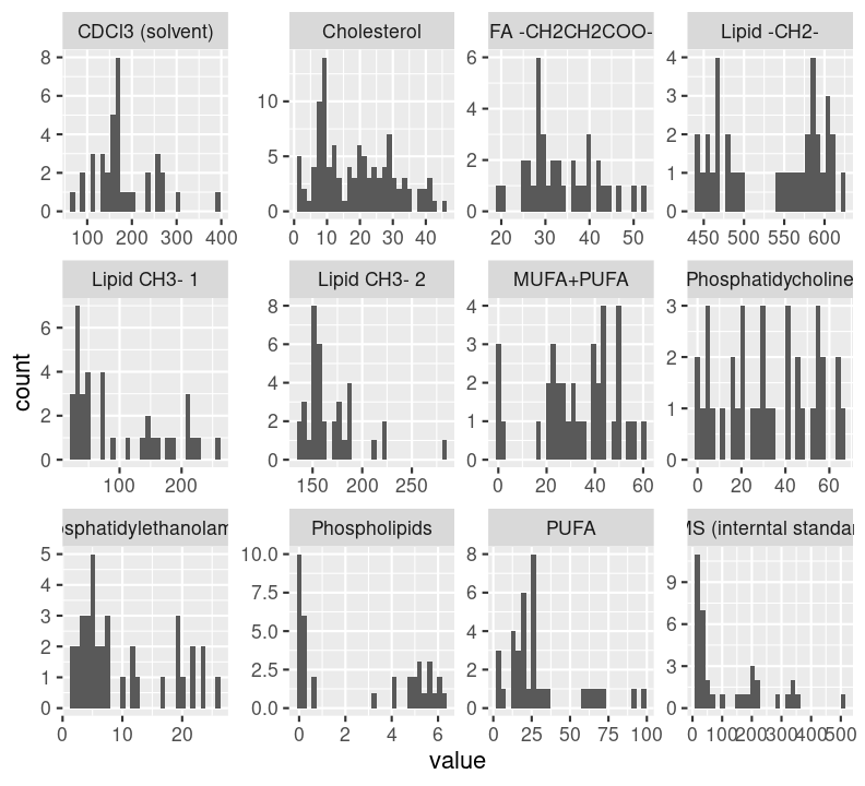
We now have the basic code to convert over into functions.
16.8 🧑💻 Exercise: Convert the plot code to a function
Time: ~10 minutes.
For now, we will only take the code to make the distribution plot and convert it into a function. Just like you did with the descriptive_stats() function in the exercise above, complete these tasks:
-
Wrap the plot code inside
doc/learning.qmdwithfunction() {...}and name the new functionplot_distributions. Use this scaffolding code to help guide you to write the code into a function.doc/learning.qmd
plot_distributions <- function(___) { ___ } Replace
lipidomicswithdataand putdataas an argument inside the brackets offunction().Add
ggplot2::to the start of each ggplot2 function used inside your function.Style using the Palette (Ctrl-Shift-PCtrl-Shift-P, then type “style file”) to make sure it is formatted correctly. You might need to manually force a styling if lines are too long.
With the cursor inside the function, add some roxygen documentation with Ctrl-Shift-Alt-RCtrl-Shift-Alt-R or with the Palette (Ctrl-Shift-PCtrl-Shift-P, then type “roxygen comment”). Remove the lines that contain
@examplesand@export, then fill in the other details (like the@paramsandTitle). In the@returnsection, write “A plot object.”Cut and paste the function over into the
R/functions.Rfile.Source the
R/functions.Rfile (Ctrl-Shift-SCtrl-Shift-S or with the Palette (Ctrl-Shift-PCtrl-Shift-P, then type “source”)) and then test the code by runningplot_distributions(lipidomics)in the Console. If it works, do the last task.Save both files and then open the Git interface and commit the changes you made to them with Ctrl-Alt-MCtrl-Alt-M or with the Palette (Ctrl-Shift-PCtrl-Shift-P, then type “commit”).
Click for the solution. Only click if you are struggling or are out of time.
## This should be in the R/functions.R file.
#' Plot for basic distribution of metabolite data.
#'
#' @param data The lipidomics dataset.
#'
#' @return A ggplot2 graph.
#'
plot_distributions <- function(data) {
data |>
ggplot2::ggplot(ggplot2::aes(x = value)) +
ggplot2::geom_histogram() +
ggplot2::facet_wrap(ggplot2::vars(metabolite), scales = "free")
}16.9 Adding the plot function as pipeline targets
Now, let’s add the plot function to the _targets.R file. Let’s write this tar_target() item within the list() inside _targets.R. To make it easier to track things, add fig_ to the start of the name given.
targets.R
list(
...,
tar_target(
name = fig_metabolite_distribution,
command = plot_distributions(lipidomics)
)
)First, style the file using the Palette (Ctrl-Shift-PCtrl-Shift-P, then type “style file”). Next, test that it works by running targets::tar_visnetwork() using the Palette (Ctrl-Shift-PCtrl-Shift-P, then type “targets visual”) or running targets::tar_outdated() with the Palette (Ctrl-Shift-PCtrl-Shift-P, then type “targets outdated”). You should see that the new item is “outdated”. Then run targets::tar_make() using the Palette (Ctrl-Shift-PCtrl-Shift-P, then type “targets run”) to update the pipeline. If it all works, than commit the changes to the Git history with Ctrl-Alt-MCtrl-Alt-M or with the Palette (Ctrl-Shift-PCtrl-Shift-P, then type “commit”).
16.10 Incorporating Quarto targets
Last, but not least, we want to make the final output 3 from ?fig-pipeline-schematic: The Quarto document. Adding a Quarto document as a target inside _targets.R is fairly straightforward. We need to install the helper package tarchetypes first, as well as the quarto R package (it helps connect with Quarto):
Console
use_package("tarchetypes")
use_package("quarto")Then, inside _targets.R, uncomment the line where library(tarchetypes) is commented out. The function we need to use to build the Quarto file is tar_quarto() (or tar_render() for R Markdown files), which needs two things: The name, like tar_target() needs, and the file path to the Quarto file. Again, like the other tar_target() items, add it to the end of the list(). Lets add doc/learning.qmd as a pipeline step:
targets.R
list(
...,
tar_quarto(
name = quarto_doc,
path = "doc/learning.qmd"
)
)Then, style the file using the Palette (Ctrl-Shift-PCtrl-Shift-P, then type “style file”). Now when we run targets::tar_make() with the Palette (Ctrl-Shift-PCtrl-Shift-P, then type “targets run”), the Quarto file also gets re-built. But when we use targets::tar_visnetwork() using the Palette (Ctrl-Shift-PCtrl-Shift-P, then type “targets visual”), we don’t see the connections with plot and descriptive statistics. That’s because we haven’t used them in a way targets can recognize. For that, we need to use the function targets::tar_read(). But because our Quarto file is located in the doc/ folder and since targets by default looks in the current folder for the targets “store” (stored objects that targets::tar_read() looks for) that is kept in the _targets/ folder, when we render the Quarto file it won’t find the store. So we have to tell targets where it is located by using targets::tar_config_set().
Let’s open up the doc/learning.qmd file, add a setup code chunk below the YAML header, and create a new header and code chunk and make use of the targets::tar_read().
doc/learning.qmd
---
# YAML header
---
```{r setup}
targets::tar_config_set(store = here::here("_targets"))
library(tidyverse)
library(targets)
source(here::here("R/functions.R"))
lipidomics <- tar_read(lipidomics)
```
## Results
```{r}
tar_read(df_stats_by_metabolite)
```
```{r}
tar_read(fig_metabolite_distribution)
```When we use targets::tar_config_set(store = ...), it will create a new file in the doc/ folder called _targets.yaml that contains details for telling targets where to find the store. Since the path listed in this new file is an absolute path, it will only ever work on your own computer. So, it improve reproducibility, it’s good practice to not put it into the Git history and instead put it in the .gitignore file. So let’s add it to ignore file by using:
Console
use_git_ignore("_targets.yaml")Before continuing, let’s commit these changes to the Git history with Ctrl-Alt-MCtrl-Alt-M or with the Palette (Ctrl-Shift-PCtrl-Shift-P, then type “commit”).
Now, going back to the doc/learning.qmd file, by using targets::tar_read(), we can access all the stored target items using syntax like we would with dplyr, without quotes. For the df_stats_by_metabolite, we can do some minor wrangling with mutate() and glue::glue(), and than pipe it to knitr::kable() to create a table in the output document. The glue package is really handy for formatting text based on columns. If you use {} inside a quoted string, you can use columns from a data frame, like value_mean. So we can use it to format the final table text to be mean value (SD value):
| Metabolite | Mean (SD) |
|---|---|
| CDCl3 (solvent) | 180 (67) |
| Cholesterol | 18.6 (11.4) |
| FA -CH2CH2COO- | 33.6 (7.8) |
| Lipid -CH2- | 536.6 (61.9) |
| Lipid CH3- 1 | 98.3 (73.8) |
| Lipid CH3- 2 | 168.2 (29.2) |
| MUFA+PUFA | 32.9 (16.1) |
| PUFA | 30 (24.1) |
| Phosphatidycholine | 31.7 (20.5) |
| Phosphatidylethanolamine | 10 (7.6) |
| Phospholipids | 2.7 (2.6) |
| TMS (internal standard) | 123 (130.4) |
Rerun targets::tar_visnetwork() using the Palette (Ctrl-Shift-PCtrl-Shift-P, then type “targets visual”) to see that it now detects the connections between the pipeline targets. Then, run targets::tar_make() with the Palette (Ctrl-Shift-PCtrl-Shift-P, then type “targets run”) again to see everything re-build! Last things are to re-style using the Palette (Ctrl-Shift-PCtrl-Shift-P, then type “style file”), then commit the changes to the Git history before moving on with Ctrl-Alt-MCtrl-Alt-M or with the Palette (Ctrl-Shift-PCtrl-Shift-P, then type “commit”). Then push your changes up to GitHub.
16.11 Fixing issues in the stored pipeline data
Note📖 Reading task: ~10 minutes
Sometimes you need to start from the beginning and clean everything up because there’s an issue that you can’t seem to fix. In this case, targets has a few functions to help out. Here are four that you can use to delete stuff (also described on the targets book):
tar_invalidate()-
This removes the metadata on the target in the pipeline, but doesn’t remove the object itself (which
tar_delete()does). This will tell targets that the target is out of date, since it has been removed, even though the data object itself isn’t present. You can use this like you wouldselect(), by naming the objects directly or using the tidyselect helpers (e.g.everything(),starts_with()). tar_delete()-
This deletes the stored objects (e.g. the
lipidomicsordf_stats_by_metabolite) inside_targets/, but does not delete the record in the pipeline. So targets will see that the pipeline doesn’t need to be rebuilt. This is useful if you want to remove some data because it takes up a lot of space, or, in the case of GDPR and privacy rules, you don’t want to store any sensitive personal health data in your project. Use it liketar_invalidate(), with functions likeeverything()orstarts_with(). tar_prune()-
This function is useful to help clean up left over or unused objects in the
_targets/folder. You will probably not use this function too often. tar_destroy()-
The most destructive, and probably more commonly used, function. This will delete the entire
_targets/folder for those times when you want to start over and rerun the entire pipeline again.
16.12 Summary
- Use a function-oriented workflow together with targets to build your data analysis pipeline and track your pipeline “targets”.
- List individual “pipeline targets” using
tar_target()within the_targets.Rfile. - Visualize target items in your pipeline with
targets::tar_visnetwork()or list outdated items withtargets::tar_outdated(). - Within R Markdown / Quarto files, use
targets::tar_read()to access saved pipeline outputs. To include the Quarto in the pipeline, use tarchetypes and the functiontar_quarto(). - Delete stored pipeline output with
tar_delete().
16.13 Code used in session
This lists some, but not all, of the code used in the section. Some code is incorporated into Markdown content, so is harder to automatically list here in a code chunk. The code below also includes the code from the exercises.
use_package("targets")
targets::use_targets()
use_package("tidyverse", "depends")
# In the {r basic-stats} chunk
lipidomics |>
  group_by(metabolite) |>
  summarise(across(value, list(mean = mean, sd = sd))) |>
  mutate(across(where(is.numeric), ~ round(.x, digits = 1)))
#' Calculate descriptive statistics of each metabolite.
#'
#' @param data The lipidomics dataset.
#'
#' @return A data.frame/tibble.
#'
descriptive_stats <- function(data) {
  data |>
    dplyr::group_by(metabolite) |>
    dplyr::summarise(dplyr::across(value, list(mean = mean, sd = sd))) |>
    dplyr::mutate(dplyr::across(tidyselect::where(is.numeric), ~ round(.x, digits = 1)))
}
list(
  tar_target(
    name = lipidomics,
    command = readr::read_csv(here::here("data/lipidomics.csv"))
  ),
  tar_target(
    name = df_stats_by_metabolite,
    command = descriptive_stats(lipidomics)
  )
)
targets::tar_make()
list(
  tar_target(
    name = file,
    command = "data/lipidomics.csv",
    format = "file"
  ),
  tar_target(
    name = lipidomics,
    command = readr::read_csv(file, show_col_types = FALSE)
  ),
  tar_target(
    name = df_stats_by_metabolite,
    command = descriptive_stats(lipidomics)
  )
)
targets::tar_visnetwork()
targets::tar_outdated()
use_package("ggplot2")
metabolite_distribution_plot <- ggplot(lipidomics, aes(x = value)) +
  geom_histogram() +
  facet_wrap(vars(metabolite), scales = "free")
metabolite_distribution_plot
## This should be in the R/functions.R file.
#' Plot for basic distribution of metabolite data.
#'
#' @param data The lipidomics dataset.
#'
#' @return A ggplot2 graph.
#'
plot_distributions <- function(data) {
  data |>
    ggplot2::ggplot(ggplot2::aes(x = value)) +
    ggplot2::geom_histogram() +
    ggplot2::facet_wrap(ggplot2::vars(metabolite), scales = "free")
}
#' Calculate descriptive statistics of each metabolite.
#'
#' @param data Lipidomics dataset.
#'
#' @return A data.frame/tibble.
#'
descriptive_stats <- function(data) {
  data |>
    dplyr::group_by(metabolite) |>
    dplyr::summarise(dplyr::across(value, list(
      mean = mean,
      sd = sd,
      median = median,
      iqr = IQR
    ))) |>
    dplyr::mutate(dplyr::across(tidyselect::where(is.numeric), ~ round(.x, digits = 1)))
}
use_package("tarchetypes")
use_package("quarto")
use_git_ignore("_targets.yaml")
targets::tar_read(df_stats_by_metabolite) |>
  mutate(MeanSD = glue::glue("{value_mean} ({value_sd})")) |>
  select(Metabolite = metabolite, `Mean SD` = MeanSD) |>
  knitr::kable(caption = "Descriptive statistics of the metabolites.")