Before beginning, get them to recall what they remember of the previous session, either with something like Mentimeter, verbally, or using hands / stickies / origami hats. Preferably something that will allow everyone to participate, not just the ones who are more comfortable being vocal to the whole group.
Depending on what they write, you may need to briefly go over the previous session.
Rarely do we run only one single statistical model to answer one single question, especially in our data-overflowing environments. An initial instinct when faced with this task might be to copy-and-paste, then slightly modify the code each time. Or, if you have heard of loops or used them in other programming languages, you might think to create a loop. Thankfully R uses something more powerful and expressive than either of those approaches, and that is functional programming. Using functional programming concepts, we can use little code to express complex actions and run large numbers of statistical analyses. This session will be about using functional programming in the context of statistical analysis.
18.1 Learning objectives
This session’s overall learning outcome is to:
Describe the basic framework underlying most statistical analyses and use R to generate statistical results using this framework.
Specific objectives are to:
Recall principles of functional programming and apply them to running statistical analyses by using the purrr package.
Continue applying the concepts and functions used from the previous sessions.
18.2 Apply logistic regression to each metabolite with functional programming
Note📖 Reading task: ~10 minutes
Functional programming underlies many core features of running statistical methods on data. Because it is such an important component of this session, you’ll briefly review the concepts of functional programming by going to the Function Programming in the Intermediate R workshop (only the reading task section) as well as the split-apply-combine (this is a short section).
TipFinished? 👒
When you’re ready to continue, place the sticky/paper hat on your computer to indicate this to the instructor 👒🎩
Note🧑🏫 Instructor note
Reinforce the concept of functional programming by briefly going over the figure that visualizes functionals like map().
There are many ways that you can run a model on each metabolite based on the lipidomics_wide dataset. However, these types of “split-apply-combine” tasks are (usually) best done using data in the long form. So we’ll start with the original lipidomics dataset. Create a header and code chunk at the end of the doc/learning.qmd file:
doc/learning.qmd
## Running multiple models```{r}```
The first thing we want to do is convert the metabolite names into snake case:
# A tibble: 504 × 6
   code   gender   age class metabolite                value
   <chr>  <chr>  <dbl> <chr> <chr>                     <dbl>
 1 ERI109 M         25 CT    tms_internal_standard    208.
 2 ERI109 M         25 CT    cholesterol               19.8
 3 ERI109 M         25 CT    lipid_ch_3_1              44.1
 4 ERI109 M         25 CT    lipid_ch_3_2             147.
 5 ERI109 M         25 CT    cholesterol               27.2
 6 ERI109 M         25 CT    lipid_ch_2               587.
 7 ERI109 M         25 CT    fa_ch_2_ch_2_coo          31.6
 8 ERI109 M         25 CT    pufa                      29.0
 9 ERI109 M         25 CT    phosphatidylethanolamine   6.78
10 ERI109 M         25 CT    phosphatidycholine        41.7
# ℹ 494 more rows
The next step is to split the data up. We could use group_by(), but in order to make the most use of purrr functions like map(), we will use group_split() to convert the data frame into a set of lists1. Let’s first add purrr as a dependency:
1 There is probably a more computationally efficient way of coding this instead of making a list, but as the saying goes “premature optimization is the root of all evil”. For our purposes, this is a very good approach, but for very large datasets and hundreds of potential models to run, this method would need to be optimized some more.
Console
use_package("purrr")
Then we run group_split() on the metabolite column, which will output a lot of data frames as a list. The website only shows the first three.
<list_of<
  tbl_df<
    code      : character
    gender    : character
    age       : double
    class     : character
    metabolite: character
    value     : double
  >
>[3]>
[[1]]
# A tibble: 36 × 6
   code   gender   age class metabolite      value
   <chr>  <chr>  <dbl> <chr> <chr>           <dbl>
 1 ERI109 M         25 CT    cd_cl_3_solvent  166.
 2 ERI111 M         39 CT    cd_cl_3_solvent  171.
 3 ERI163 W         58 CT    cd_cl_3_solvent  262.
 4 ERI375 M         24 CT    cd_cl_3_solvent  172.
 5 ERI376 M         26 CT    cd_cl_3_solvent  300.
 6 ERI391 M         31 CT    cd_cl_3_solvent  241.
 7 ERI392 M         24 CT    cd_cl_3_solvent  172.
 8 ERI79  W         26 CT    cd_cl_3_solvent  148.
 9 ERI81  M         52 CT    cd_cl_3_solvent  168.
10 ERI83  M         25 CT    cd_cl_3_solvent  253.
# ℹ 26 more rows

[[2]]
# A tibble: 108 × 6
   code   gender   age class metabolite  value
   <chr>  <chr>  <dbl> <chr> <chr>       <dbl>
 1 ERI109 M         25 CT    cholesterol 19.8
 2 ERI109 M         25 CT    cholesterol 27.2
 3 ERI109 M         25 CT    cholesterol  8.88
 4 ERI111 M         39 CT    cholesterol 22.8
 5 ERI111 M         39 CT    cholesterol 30.2
 6 ERI111 M         39 CT    cholesterol  9.28
 7 ERI163 W         58 CT    cholesterol 14.9
 8 ERI163 W         58 CT    cholesterol 24.0
 9 ERI163 W         58 CT    cholesterol  7.66
10 ERI375 M         24 CT    cholesterol 19.2
# ℹ 98 more rows

[[3]]
# A tibble: 36 × 6
   code   gender   age class metabolite       value
   <chr>  <chr>  <dbl> <chr> <chr>            <dbl>
 1 ERI109 M         25 CT    fa_ch_2_ch_2_coo  31.6
 2 ERI111 M         39 CT    fa_ch_2_ch_2_coo  28.9
 3 ERI163 W         58 CT    fa_ch_2_ch_2_coo  36.6
 4 ERI375 M         24 CT    fa_ch_2_ch_2_coo  39.4
 5 ERI376 M         26 CT    fa_ch_2_ch_2_coo  52.1
 6 ERI391 M         31 CT    fa_ch_2_ch_2_coo  42.8
 7 ERI392 M         24 CT    fa_ch_2_ch_2_coo  39.9
 8 ERI79  W         26 CT    fa_ch_2_ch_2_coo  32.7
 9 ERI81  M         52 CT    fa_ch_2_ch_2_coo  28.4
10 ERI83  M         25 CT    fa_ch_2_ch_2_coo  26.5
# ℹ 26 more rows
Remember that logistic regression models need each row to be a single person, so we’ll use the functional map() to apply our custom function metabolites_to_wider() on each of the split list items (only showing the first three):
[[1]]
# A tibble: 36 × 5
   code   gender   age class metabolite_cd_cl_3_solvent
   <chr>  <chr>  <dbl> <chr>                      <dbl>
 1 ERI109 M         25 CT                          166.
 2 ERI111 M         39 CT                          171.
 3 ERI163 W         58 CT                          262.
 4 ERI375 M         24 CT                          172.
 5 ERI376 M         26 CT                          300.
 6 ERI391 M         31 CT                          241.
 7 ERI392 M         24 CT                          172.
 8 ERI79  W         26 CT                          148.
 9 ERI81  M         52 CT                          168.
10 ERI83  M         25 CT                          253.
# ℹ 26 more rows

[[2]]
# A tibble: 36 × 5
   code   gender   age class metabolite_cholesterol
   <chr>  <chr>  <dbl> <chr>                  <dbl>
 1 ERI109 M         25 CT                     18.6
 2 ERI111 M         39 CT                     20.8
 3 ERI163 W         58 CT                     15.5
 4 ERI375 M         24 CT                     10.2
 5 ERI376 M         26 CT                     13.5
 6 ERI391 M         31 CT                      9.53
 7 ERI392 M         24 CT                      9.87
 8 ERI79  W         26 CT                     17.6
 9 ERI81  M         52 CT                     17.0
10 ERI83  M         25 CT                     19.7
# ℹ 26 more rows

[[3]]
# A tibble: 36 × 5
   code   gender   age class metabolite_fa_ch_2_ch_2_coo
   <chr>  <chr>  <dbl> <chr>                       <dbl>
 1 ERI109 M         25 CT                           31.6
 2 ERI111 M         39 CT                           28.9
 3 ERI163 W         58 CT                           36.6
 4 ERI375 M         24 CT                           39.4
 5 ERI376 M         26 CT                           52.1
 6 ERI391 M         31 CT                           42.8
 7 ERI392 M         24 CT                           39.9
 8 ERI79  W         26 CT                           32.7
 9 ERI81  M         52 CT                           28.4
10 ERI83  M         25 CT                           26.5
# ℹ 26 more rows
Alright, we now a list of data frames where each data frame has only one of the metabolites. These bits of code represent the conceptual action of “splitting the data into a list by metabolites”. Since we’re following a function-oriented workflow, let’s create a function for this. Convert it into a function, add the Roxygen documentation using Ctrl-Shift-Alt-RCtrl-Shift-Alt-R or with the Palette (Ctrl-Shift-PCtrl-Shift-P, then type “roxygen comment”) style using the Palette (Ctrl-Shift-PCtrl-Shift-P, then type “style file”), move into the R/functions.R file, and then source() the file with Ctrl-Shift-SCtrl-Shift-S or with the Palette (Ctrl-Shift-PCtrl-Shift-P, then type “source”).
R/functions.R
#' Convert the long form dataset into a list of wide form data frames.#'#' @param data The lipidomics dataset.#'#' @return A list of data frames.#'split_by_metabolite<-function(data){data|>column_values_to_snake_case(metabolite)|>dplyr::group_split(metabolite)|>purrr::map(metabolites_to_wider)}
In the doc/learning.qmd, use the new function in the code:
doc/learning.qmd
lipidomics|>split_by_metabolite()
[[1]]
# A tibble: 36 × 5
   code   gender   age class metabolite_cd_cl_3_solvent
   <chr>  <chr>  <dbl> <chr>                      <dbl>
 1 ERI109 M         25 CT                          166.
 2 ERI111 M         39 CT                          171.
 3 ERI163 W         58 CT                          262.
 4 ERI375 M         24 CT                          172.
 5 ERI376 M         26 CT                          300.
 6 ERI391 M         31 CT                          241.
 7 ERI392 M         24 CT                          172.
 8 ERI79  W         26 CT                          148.
 9 ERI81  M         52 CT                          168.
10 ERI83  M         25 CT                          253.
# ℹ 26 more rows

[[2]]
# A tibble: 36 × 5
   code   gender   age class metabolite_cholesterol
   <chr>  <chr>  <dbl> <chr>                  <dbl>
 1 ERI109 M         25 CT                     18.6
 2 ERI111 M         39 CT                     20.8
 3 ERI163 W         58 CT                     15.5
 4 ERI375 M         24 CT                     10.2
 5 ERI376 M         26 CT                     13.5
 6 ERI391 M         31 CT                      9.53
 7 ERI392 M         24 CT                      9.87
 8 ERI79  W         26 CT                     17.6
 9 ERI81  M         52 CT                     17.0
10 ERI83  M         25 CT                     19.7
# ℹ 26 more rows

[[3]]
# A tibble: 36 × 5
   code   gender   age class metabolite_fa_ch_2_ch_2_coo
   <chr>  <chr>  <dbl> <chr>                       <dbl>
 1 ERI109 M         25 CT                           31.6
 2 ERI111 M         39 CT                           28.9
 3 ERI163 W         58 CT                           36.6
 4 ERI375 M         24 CT                           39.4
 5 ERI376 M         26 CT                           52.1
 6 ERI391 M         31 CT                           42.8
 7 ERI392 M         24 CT                           39.9
 8 ERI79  W         26 CT                           32.7
 9 ERI81  M         52 CT                           28.4
10 ERI83  M         25 CT                           26.5
# ℹ 26 more rows
Like we did with the metabolite_to_wider(), we need to pipe the output into another map() function that has a custom function running the models. We don’t have this function yet, so we need to create it. Let’s convert the modeling code we used in the code at the end of section Section 17.8 into a function, replacing lipidomics with data and using starts_with("metabolite_") within the create_recipe_spec(). Add the Roxygen documentation using Ctrl-Shift-Alt-RCtrl-Shift-Alt-R or with the Palette (Ctrl-Shift-PCtrl-Shift-P, then type “roxygen comment”), use the Palette (Ctrl-Shift-PCtrl-Shift-P, then type “style file”) to style, move into the R/functions.R file, and then source() the file with Ctrl-Shift-SCtrl-Shift-S or with the Palette (Ctrl-Shift-PCtrl-Shift-P, then type “source”).
R/functions.R
#' Generate the results of a model#'#' @param data The lipidomics dataset.#'#' @return A data frame.#'generate_model_results<-function(data){create_model_workflow(parsnip::logistic_reg()|>parsnip::set_engine("glm"),data|>create_recipe_spec(tidyselect::starts_with("metabolite_")))|>parsnip::fit(data)|>tidy_model_output()}
Then we add it to the end of the pipe, but using map() and list_rbind() to convert to a data frame:
Since we are only interested in the model results for the metabolites, let’s keep only the term rows that are metabolites using filter() and str_detect().
Wow! We’re basically at our first targets output! Before continuing, do an exercise to convert the code into a function.
18.3🧑💻 Exercise: Create a function to calculate the model estimates
Time: ~10 minutes.
Convert the code into a function that calculates the model estimates. Use this scaffold to help complete the tasks below for the calculate_estimates() function:
calculate_estimates <-function(data) { ___ |># Code from right before the exercise that creates the results ___}
Name the new function calculate_estimates.
Within the function(), add one argument called data.
Paste the code we created from above into the function, replacing lipidomics with data.
Add dplyr::, purrr::, and stringr:: before their respective functions.
Add the Roxygen documentation using Ctrl-Shift-Alt-RCtrl-Shift-Alt-R or with the Palette (Ctrl-Shift-PCtrl-Shift-P, then type “roxygen comment”).
Use the Palette (Ctrl-Shift-PCtrl-Shift-P, then type “style file”) to style the file to fix up the code.
Cut and paste the function over into the R/functions.R file.
Commit the changes you’ve made so far with Ctrl-Alt-MCtrl-Alt-M or with the Palette (Ctrl-Shift-PCtrl-Shift-P, then type “commit”).
Click for the solution. Only click if you are struggling or are out of time.
#' Calculate the estimates for the model for each metabolite.#'#' @param data The lipidomics dataset.#'#' @return A data frame.#'calculate_estimates<-function(data){data|>split_by_metabolite()|>purrr::map(generate_model_results)|>purrr::list_rbind()|>dplyr::filter(stringr::str_detect(term, "metabolite_"))}
TipFinished? 👒
When you’re ready to continue, place the sticky/paper hat on your computer to indicate this to the instructor 👒🎩
18.4 Improve the readability of the model output
We now have a function that calculates the model estimates, but it outputs the variable names in snake case. While this is a good practice for programming, it is not the most aesthetic for reporting. Let’s add back the original variable names, rather than the snake case version. Since the original variable still exists in our lipidomics dataset, we can join it to the model_estimates object with right_join(), along with a few other minor changes. First, we’ll select() only the metabolite and then create a duplicate column of metabolite called term (to match the model_estimates) using mutate().
Right after that we will use our custom column_values_to_snake_case() function on the term column so it matches the term variable in the model estimates data frame.
There are 504 rows, but we only need the unique values of term and metabolite, which we can get with distinct(). Because we will use distinct(), we don’t need to use select() as well, since it keeps only the metabolite and term variables.
Awesome 😄 Now let’s bring this code into the calculate_estimates() function we created. Then afterwards we can add our first targets output!
18.5🧑💻 Exercise: Incorporate additional code into an existing function
Time: ~12 minutes.
Taking the code above, we’ll insert it into the calculate_estimates() function so it has a nicer looking and more readable output. While in the R/functions.R, go to the calculate_estimates() function. Use this scaffold to help with the tasks below for adding more code to the calculate_estimates() function:
calculate_estimates <-function(data) {# 1. Assign the output to a object. ___ <- data |>split_by_metabolite() |> purrr::map(generate_model_results) |> purrr::list_rbind() |> dplyr::filter(stringr::str_detect(term, "metabolite_")) data |># 2. Add the code we created above. ___ |># 3. Include the object from the first step here.right_join(___, by ="term")}
Assign the output of the first chunk of code that creates the model estimates and name the new variable model_estimates.
Paste the code we created into the function, so that the data variable pipes into it.
Add model_estimates to the right_join() function.
Add dplyr:: and stringr:: before their respective functions.
Use the Palette (Ctrl-Shift-PCtrl-Shift-P, then type “style file”) to style the file to fix up the code.
Commit the changes you’ve made so far with Ctrl-Alt-MCtrl-Alt-M or with the Palette (Ctrl-Shift-PCtrl-Shift-P, then type “commit”).
Click for the solution. Only click if you are struggling or are out of time.
#' Calculate the estimates for the model for each metabolite.#'#' @param data The lipidomics dataset.#'#' @return A data frame.#'calculate_estimates<-function(data){model_estimates<-data|>split_by_metabolite()|>purrr::map(generate_model_results)|>purrr::list_rbind()|>dplyr::filter(stringr::str_detect(term, "metabolite_"))data|>dplyr::mutate(term =metabolite)|>column_values_to_snake_case(term)|>dplyr::mutate(term =stringr::str_c("metabolite_", term))|>dplyr::distinct(term, metabolite)|>dplyr::right_join(model_estimates, by ="term")}
TipFinished? 👒
When you’re ready to continue, place the sticky/paper hat on your computer to indicate this to the instructor 👒🎩
18.6🧑💻 Exercise: Add a target for the model results
Time: ~8 minutes
Taking the function code from above, you’ll next add the model results output to end of the _targets.R file, using the below scaffold as a guide.
Use the calculate_estimates() function in command, with lipidomics as the argument.
Use the Palette (Ctrl-Shift-PCtrl-Shift-P, then type “style file”) to style and than run targets::tar_visnetwork() using the Palette (Ctrl-Shift-PCtrl-Shift-P, then type “targets visual”) to see if the new target gets detected. If it does, than run targets::tar_make() with the Palette (Ctrl-Shift-PCtrl-Shift-P, then type “targets run”).
Commit the changes to the Git history with Ctrl-Alt-MCtrl-Alt-M or with the Palette (Ctrl-Shift-PCtrl-Shift-P, then type “commit”).
Click for the solution. Only click if you are struggling or are out of time.
list(# ...,tar_target( name =df_model_estimates, command =calculate_estimates(lipidomics)))
TipFinished? 👒
When you’re ready to continue, place the sticky/paper hat on your computer to indicate this to the instructor 👒🎩
18.7 Visualizing the model estimates
We’ve got one target done for the modeling stage, three more to go! There are multiple ways of visualizing the results from models. A common approach is to use a “dot-and-whisker” plot like you might see in a meta-analysis. Often the “whisker” part is the measure of uncertainty like the confidence interval, and the “dot” is the estimate. For the confidence interval, we haven’t calculated them at this point because the typical approach doesn’t exactly work for our data (tested before the workshop). For this plot though, we will use the standard error of the estimate.
Inside the doc/learning.qmd, let’s create a new header and code chunk inside the ## Results section. We’ll want to use tar_read(df_model_estimates) so that targets is aware that the R Markdown file is dependent on this target.
doc/learning.qmd
### Figure of model estimates```{r}model_estimates <-tar_read(df_model_estimates)```
Then we’ll start using ggplot2 to visualize the results. For dot-whisker plots, the “geom” we would use is called geom_pointrange(). It requires four values:
x: This will be the “dot”, representing the estimate column.
y: This is the categorical variable that the “dot” is associated with, in this case, it is the metabolite column.
xmin: This is the lower end of the “whisker”. Since the std.error is a value representing uncertainty of the estimate on either side of it (+ or -), we will need to subtract std.error from the estimate.
xmax: This is the upper end of the “whisker”. Like xmin above, but adding std.error instead.
doc/learning.qmd
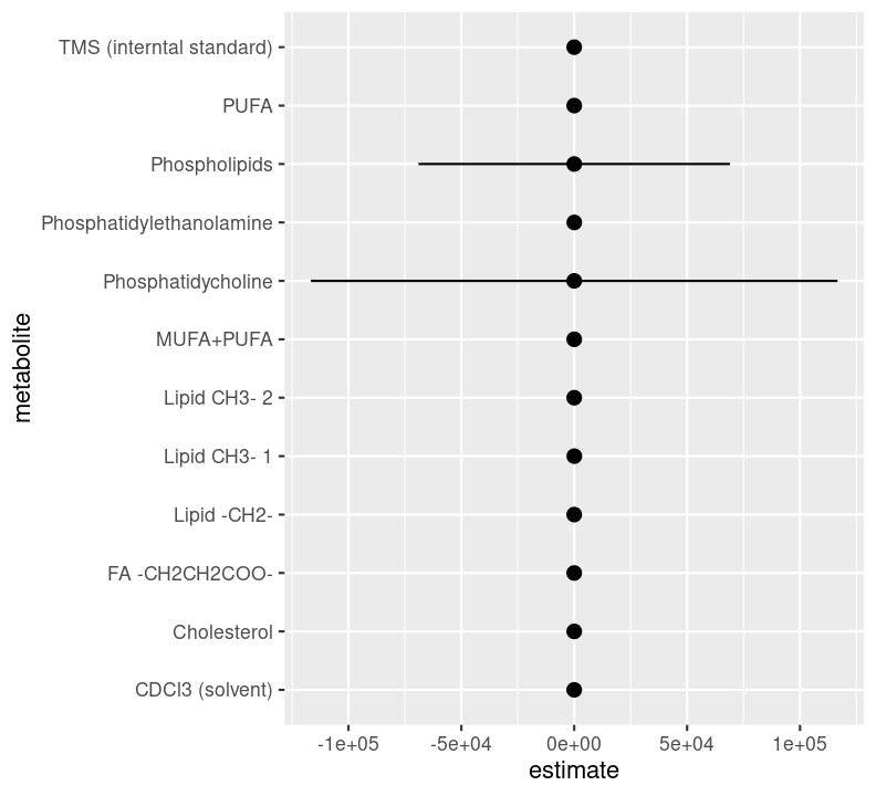
plot_estimates<-model_estimates|>ggplot(aes( x =estimate, y =metabolite, xmin =estimate-std.error, xmax =estimate+std.error))+geom_pointrange()plot_estimates
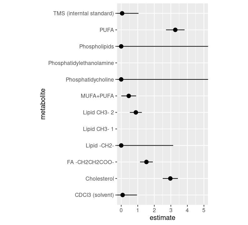
Woah, there is definitely something wrong here. The values of the estimate should realistically be somewhere between 0 (can’t have a negative odds) and 2 (in biology and health research, odds ratios are rarely above 2), definitely unlikely to be more than 5. We will eventually need to troubleshoot this issue, but for now, let’s restrict the x axis to be between 0 and 5.
There are so many things we could start investigating based on these results in order to fix them up. But for now, this will do.
18.8🧑💻 Exercise: Add plot function as a target in the pipeline
Time: ~15 minutes.
Hopefully you’ve gotten comfortable with the function-oriented workflow, because we’ll need to convert this plot code into a function and add it as a target in the pipeline. Use the scaffold below as a guide.
Move the function into the R/functions.R file, add the Roxygen documentation using Ctrl-Shift-Alt-RCtrl-Shift-Alt-R or with the Palette (Ctrl-Shift-PCtrl-Shift-P, then type “roxygen comment”), and use the Palette (Ctrl-Shift-PCtrl-Shift-P, then type “style file”) to style.
Click for the solution. Only click if you are struggling or are out of time.
#' Plot the estimates and standard errors of the model results.#'#' @param results The model estimate results.#'#' @return A ggplot2 figure.#'plot_estimates<-function(results){results|>ggplot2::ggplot(ggplot2::aes( x =estimate, y =metabolite, xmin =estimate-std.error, xmax =estimate+std.error))+ggplot2::geom_pointrange()+ggplot2::coord_fixed(xlim =c(0, 5))}
Then, after doing that, add the new function as a target in the pipeline, name the new name as fig_model_estimates. Inside the plot_estimates() function, use the the model estimate target we created previously (df_model_estimates).
Click for the solution. Only click if you are struggling or are out of time.
list(# ...,tar_target( name =fig_model_estimates, command =plot_estimates(df_model_estimates)))
TipFinished? 👒
When you’re ready to continue, place the sticky/paper hat on your computer to indicate this to the instructor 👒🎩
18.9 Combine all the output into the Quarto file
Now its’ time to add the model results and plots to the doc/learning.qmd file. Open it up and create another code chunk at the bottom of the file. Like we did with the other outputs (like the figures), we’ll use tar_read() to reference the image path.
```{r}tar_read(fig_model_estimates)```
Run targets::tar_visnetwork() using the Palette (Ctrl-Shift-PCtrl-Shift-P, then type “targets visual”), then targets::tar_make() with the Palette (Ctrl-Shift-PCtrl-Shift-P, then type “targets run”). We now have the report rendered to an HTML file! If you open it up in a browser, we can see the figures added to it. Before ending, commit the changes to the Git history with Ctrl-Alt-MCtrl-Alt-M or with the Palette (Ctrl-Shift-PCtrl-Shift-P, then type “commit”).
18.10 Summary
Use functional programming with map(), as part of the function-oriented workflow, to run multiple models efficiently and with minimal code.
Consistently create small functions that do a specific conceptual action and chain them together into larger conceptual actions, which can then more easily be incorporated into a targets pipeline. Small, multiple functions combined together are easier to manage than fewer, bigger ones.
Use dot-whisker plots like geom_pointrange() to visualize the estimates and their standard error.
18.11 Code used in session
This lists some, but not all, of the code used in the section. Some code is incorporated into Markdown content, so is harder to automatically list here in a code chunk. The code below also includes the code from the exercises.
lipidomics|>column_values_to_snake_case(metabolite)use_package("purrr")lipidomics|>column_values_to_snake_case(metabolite)|>group_split(metabolite)lipidomics|>column_values_to_snake_case(metabolite)|>group_split(metabolite)|>map(metabolites_to_wider)#' Convert the long form dataset into a list of wide form data frames.#'#' @param data The lipidomics dataset.#'#' @return A list of data frames.#'split_by_metabolite<-function(data){data|>column_values_to_snake_case(metabolite)|>dplyr::group_split(metabolite)|>purrr::map(metabolites_to_wider)}lipidomics|>split_by_metabolite()#' Generate the results of a model#'#' @param data The lipidomics dataset.#'#' @return A data frame.#'generate_model_results<-function(data){create_model_workflow(parsnip::logistic_reg()|>parsnip::set_engine("glm"),data|>create_recipe_spec(tidyselect::starts_with("metabolite_")))|>parsnip::fit(data)|>tidy_model_output()}lipidomics|>split_by_metabolite()|>map(generate_model_results)|>list_rbind()model_estimates<-lipidomics|>split_by_metabolite()|>map(generate_model_results)|>list_rbind()|>filter(str_detect(term, "metabolite_"))model_estimates#' Calculate the estimates for the model for each metabolite.#'#' @param data The lipidomics dataset.#'#' @return A data frame.#'calculate_estimates<-function(data){data|>split_by_metabolite()|>purrr::map(generate_model_results)|>purrr::list_rbind()|>dplyr::filter(stringr::str_detect(term, "metabolite_"))}lipidomics|>select(metabolite)|>mutate(term =metabolite)lipidomics|>select(metabolite)|>mutate(term =metabolite)|>column_values_to_snake_case(term)lipidomics|>select(metabolite)|>mutate(term =metabolite)|>column_values_to_snake_case(term)|>mutate(term =str_c("metabolite_", term))lipidomics|>mutate(term =metabolite)|>column_values_to_snake_case(term)|>mutate(term =str_c("metabolite_", term))|>distinct(term, metabolite)lipidomics|>mutate(term =metabolite)|>column_values_to_snake_case(term)|>mutate(term =str_c("metabolite_", term))|>distinct(term, metabolite)|>right_join(calculate_estimates(lipidomics), by ="term")#' Calculate the estimates for the model for each metabolite.#'#' @param data The lipidomics dataset.#'#' @return A data frame.#'calculate_estimates<-function(data){model_estimates<-data|>split_by_metabolite()|>purrr::map(generate_model_results)|>purrr::list_rbind()|>dplyr::filter(stringr::str_detect(term, "metabolite_"))data|>dplyr::mutate(term =metabolite)|>column_values_to_snake_case(term)|>dplyr::mutate(term =stringr::str_c("metabolite_", term))|>dplyr::distinct(term, metabolite)|>dplyr::right_join(model_estimates, by ="term")}list(# ...,tar_target( name =df_model_estimates, command =calculate_estimates(lipidomics)))plot_estimates<-model_estimates|>ggplot(aes( x =estimate, y =metabolite, xmin =estimate-std.error, xmax =estimate+std.error))+geom_pointrange()plot_estimatesplot_estimates+coord_fixed(xlim =c(0, 5))#' Plot the estimates and standard errors of the model results.#'#' @param results The model estimate results.#'#' @return A ggplot2 figure.#'plot_estimates<-function(results){results|>ggplot2::ggplot(ggplot2::aes( x =estimate, y =metabolite, xmin =estimate-std.error, xmax =estimate+std.error))+ggplot2::geom_pointrange()+ggplot2::coord_fixed(xlim =c(0, 5))}list(# ...,tar_target( name =fig_model_estimates, command =plot_estimates(df_model_estimates)))