22 Visualizing the results of many models

Effectively visualizing the results of your analysis is an important part in communicating your findings to others. We’ve created an object that contains the results from the previous session. Now we want to take that object, make a figure of it, and> include it into our pipeline and Quarto report.

22.1 Learning objectives

Use an effective way to visualise the results from multiple statistical models fitted to different subsets of data using the ggplot2 R package.
Identify how a fully reproducible analysis pipeline looks like, from start to finish, and how this workflow might make a data analysis project easier for you and your collaborators to work on together.

22.2 📖 Reading task: Understanding the model output

Time: ~10 minutes.

Let’s explain this output a bit, each column at a time. You don’t have to read about the metabolite and model columns that we added in the previous sessions, since you added them yourselves. Both are columns to help you identify what results are for which metabolite and model. But the other columns you may not be familiar with:

term: This column contains all the predictor variables found within the model you used, including the intercept (if you recall from Chapter 19 that it is part of the regression formula). So the number of term rows should be at least as many rows as there are predictor variables in the model. For example, if your model is $c l a s s = v a l u e + a g e + g e n d e r$ , there will be a row in term with value, age, and gender. You notice that there is no row for class. That’s because class is the outcome variable, not a predictor variable. The values in estimate are used with the values of the predictor variables to predict what the value of class might be.
estimate: This column is the “coefficient” linked to the term in the model. The final mathematical model here looks like:

$\begin{matrix} c l a s s = i n t e r c e p t + (v a l u e_e s t i m a t e \times v a l u e_n u m b e r) + \\ (g e n d e r_e s t i m a t e \times g e n d e r_n u m b e r) + . . . \end{matrix}$

In our example, we chose to get the odds ratios. In the mathematical model above, the estimate is represented as the log odds ratio or beta coefficient—the constant value you multiply the value of the term with. Interpreting each of these values can be quite tricky and can take a surprising amount of time to conceptually break down, so we won’t do that here, since this isn’t a statistics workshop. The only thing you need to understand here is that the estimate is the value that tells us the magnitude of association between the term and class. This value, along with the std.error are the most important values we can get from the model and we will be using them when presenting the results.
std.error: This is the uncertainty in the estimate value. A higher value means there is less certainty in the value of the estimate. This number, combined with the estimate, are what we usually actually want to know about: “how big is the effect and how certain are we about it?”
statistic: This value is used to determine the p.value. We don’t need it, nor will we use it in this workshop.
p.value: This is the infamous value we researchers are obsessed about and can think nothing else of. While there is a lot of attention to this single value, there are a large number of issues with using and in particular interpreting it. You can learn more about it in the statement about it from the American Statistical Association. We won’t cover this particular topic in this workshop, aside from stating that the interpretation of the p-value is very difficult and very much misused. Meanwhile, the estimate is a lot easier to understand, interpret, and explain. And most of the time, this is the value that we actually care about because it represents the magnitude of impact that a predictor has on an outcome. Because of this, we won’t use or work with the p.value in the rest of this workshop.

Sticky/hat up!

When you’re ready to continue, place the sticky/paper hat on your computer to indicate this to the teacher 👒 🎩

22.3 Building up the graph

Often results from models are presented in a table format. However, visualizing them is a lot more effective at showing potential insights and interesting patterns, as well as communicating the results to others. In this section, we will create a simple visualization of the model results we generated in the previous session. If we return to our pipeline diagram from before, we’ve completed the model_results target, and now need to create the plot_model_results target. This means we want to create the function create_plot_model_results() that will take the model_results data frame and create a plot from it.

Figure 22.1: The last remaining target… plotting the model results!

There are many ways of visualizing the results from models. A common approach is to use a “dot-and-whisker” plot like you might see in a meta-analysis. Often the “whisker” part is the measure of uncertainty like the confidence interval, and the “dot” is the estimate. We didn’t calculate the confidence interval because it often requires more extensive checks of the data and of model assumptions to do properly. In fact, while developing the material for this workshop and trying to include the confidence interval, the code didn’t run because of issues with the data. Investigating the issue during the workshop would require doing checks that are well beyond the scope of this workshop. So instead, we will just use the standard error.

Go into the docs/learning.qmd and create a new header and code chunk right above the ## Appendix header we created previously. Since we ran the targets pipeline with the model_results previously, we should have it available to us via tar_read(). So in the new code chunk, we will read in the model results using it:

docs/learning.qmd

### Figure of model estimates

```{r}
model_results <- tar_read(model_results)
```

🧑‍🏫 Teacher note

Verbally explain each point below, though you don’t need to show the website during this part. You can rely on reading it from your print-out, cell, or pad.

There’s a lot of information here and there’s many things we could potential visualize. Let’s break it down.

We need the estimate and the std.error columns in order to plot the dot and whisker plot, since the estimate is the dot and the std.error is used to create the whisker.
We need to know which metabolite the results come from so we can properly label our plot. Maybe we could put the metabolite on the y axis, so that the dots are aligned vertically for each metabolite.
We might also want the model column if we want to show results from both models. In this case, we could have the models be shown on top of each other for each metabolite or we could have separate plots for each model.
We probably don’t need all the rows that are in the results data frame, which are listed in the term column. At least for our research questions, we really only want the estimates for the metabolites and not for the variables gender or age. In this case, we only need the rows where term is value.

🧑‍🏫 Teacher note

For this next part, slowly build up the code, explaining each step after a pipe or after a ggplot layer is added. You can continue to build off of the same code in the same code chunk rather than make new code chunks each time.

So to start we will filter() and then select() the data we want:

docs/learning.qmd

model_results |>
  filter(term == "value") |>
  select(metabolite, model, estimate, std.error)

# A tibble: 24 × 4
   metabolite      model                        estimate std.error
   <chr>           <chr>                           <dbl>     <dbl>
 1 CDCl3 (solvent) class ~ value                 0.112       0.818
 2 CDCl3 (solvent) class ~ value + gender + age  0.0870      0.865
 3 Cholesterol     class ~ value                 2.65        0.450
 4 Cholesterol     class ~ value + gender + age  2.97        0.458
 5 FA -CH2CH2COO-  class ~ value                 1.43        0.351
 6 FA -CH2CH2COO-  class ~ value + gender + age  1.52        0.387
 7 Lipid -CH2-     class ~ value                 0.0172      1.53 
 8 Lipid -CH2-     class ~ value + gender + age  0.00259     3.14 
 9 Lipid CH3- 1    class ~ value                40.7         1.35 
10 Lipid CH3- 1    class ~ value + gender + age 44.5         1.41 
# ℹ 14 more rows

Great! Ok, now we can start plotting the results!

Then we’ll start using ggplot2 to visualize the results. For dot-whisker plots, the “geom” we would use is called geom_pointrange(). It requires four values:

x: This will be the “dot”, representing the estimate column.
y: This is the categorical variable that the “dot” is associated with, in this case, it is the metabolite column.
xmin: This is the lower end of the “whisker”. Since the std.error is a value representing uncertainty of the estimate on either side of it (+ or -), we will need to subtract std.error from the estimate.
xmax: This is the upper end of the “whisker”. Like xmin above, but adding std.error instead.

Let’s make this plot! In our case, because we had research questions that involve the two models, but that we aren’t comparing them directly, we can use facet_grid() to show the two models separately. We’ll facet so they are side-by-side rather than on top of each other, so we will use cols = vars(model). We can also add a vertical line at x = 1, since an odds ratio of 1 means “no effect” by using the geom_vline() function with the xintercept argument. We’ll use a dashed line type to make it less visually prominent.

docs/learning.qmd

model_results |>
  filter(term == "value") |>
  select(metabolite, model, estimate, std.error) |>
  ggplot(aes(
    x = estimate,
    y = metabolite,
    xmin = estimate - std.error,
    xmax = estimate + std.error
  )) +
  geom_pointrange() +
  geom_vline(xintercept = 1, linetype = "dashed") +
  facet_grid(cols = vars(model))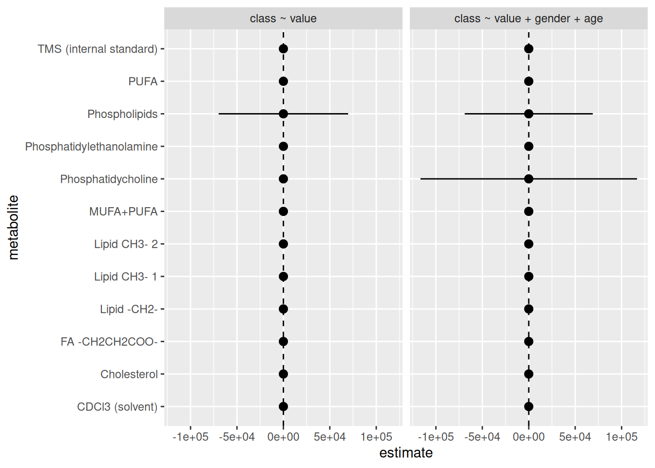

Woah, there is definitely something wrong here. There’s something very wrong with the standard error values of some metabolites. Some of them are huge! So let’s fix this standard error issue. In a real analyses, we would go back to the data and the models to figure out what is wrong. It is likely that there are some data quality issues or that the variability within the data itself is just too high for these variables. Either way, this is outside the scope of this workshop. So instead, we will just drop those values so we don’t plot them. So, let’s remove any std.error values that are above maybe 2, since that already is quite large of a standard error. We’ll do that in the filter() step.

docs/learning.qmd

model_results |>
  filter(term == "value", std.error <= 2) |>
  select(metabolite, model, estimate, std.error) |>
  ggplot(aes(
    x = estimate,
    y = metabolite,
    xmin = estimate - std.error,
    xmax = estimate + std.error
  )) +
  geom_pointrange() +
  geom_vline(xintercept = 1, linetype = "dashed") +
  facet_grid(cols = vars(model))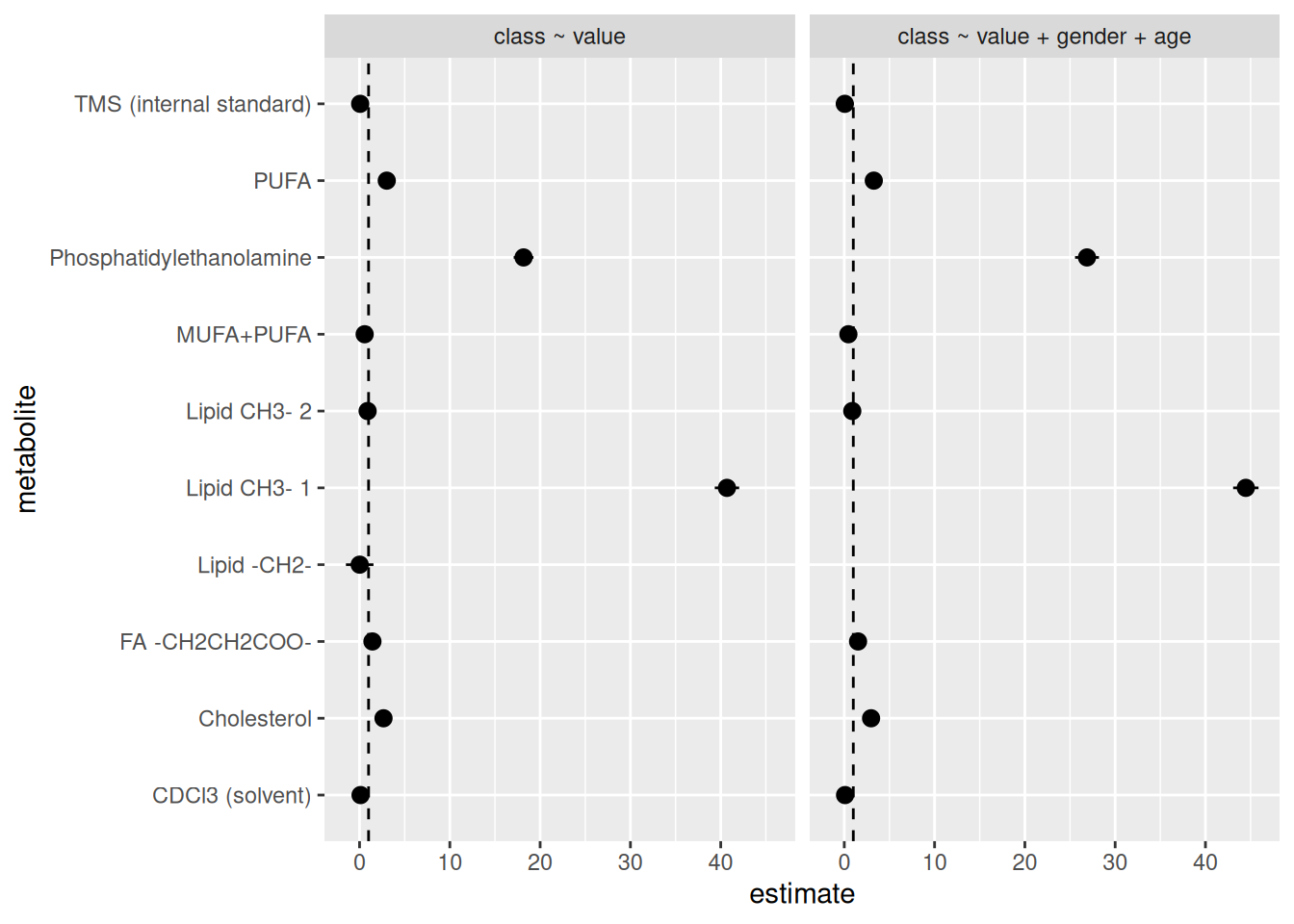

We see it dropped some metabolites. But there’s still an issue. Some of the metabolites have estimate values that are huge! Way too big to be realistic or a real result. The values of the estimates should realistically be somewhere between 0 (it’s not possible to have an odds ratio be negative) and 2 (in biology and health research, odds ratios are rarely above 2), definitely unlikely to be more than 5. To put that into perspective, odds ratio above a 4 is already considered quite large in biology and health research and that really only occurs when there is a strong causal relationship between the predictor and the outcome. In the case of the biology between a specific metabolite and type 1 diabetes status, the odds ratio will be much closer to 1. So for this workshop, let’s just filter out any estimate values above 5, to be generous with the cutoff.

docs/learning.qmd

model_results |>
  filter(term == "value", std.error <= 2, estimate <= 5) |>
  select(metabolite, model, estimate, std.error) |>
  ggplot(aes(
    x = estimate,
    y = metabolite,
    xmin = estimate - std.error,
    xmax = estimate + std.error
  )) +
  geom_pointrange() +
  geom_vline(xintercept = 1, linetype = "dashed") +
  facet_grid(cols = vars(model))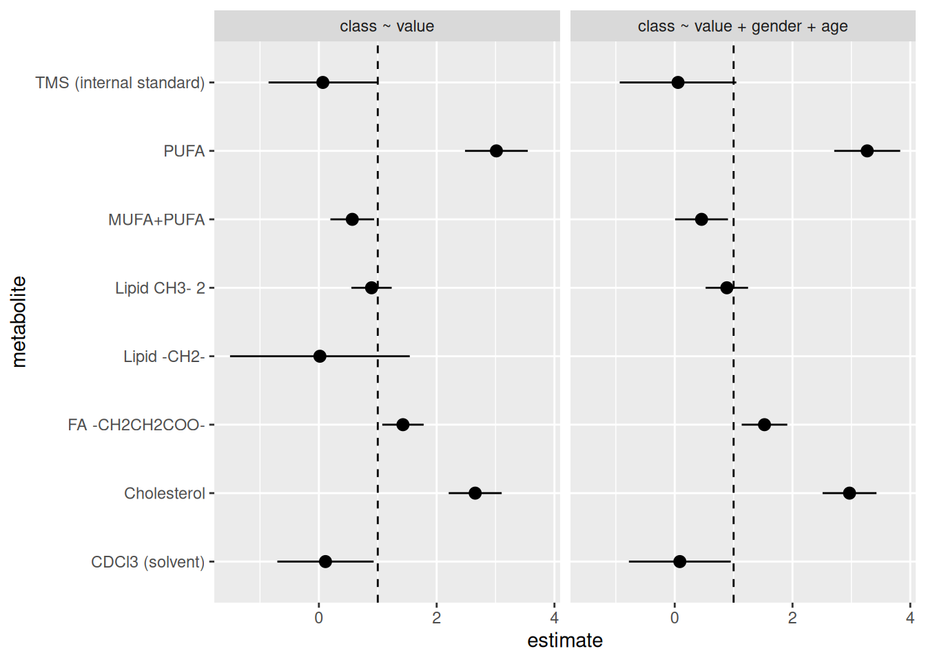

There are so many things we could start investigating based on these results in order to fix them up. But for now, this will do. Let’s style the code with the Palette (Ctrl-Shift-P, then type “style file”) and then commit to the Git history with Ctrl-Alt-M or with the Palette (Ctrl-Shift-P, then type “commit”) before pushing to GitHub.

22.4 🧑‍💻 Exercise: Convert the plot code into a function

Time: ~8 minutes.

This is the last function to create for our pipeline! Use the scaffold below as a guide to convert the code we just wrote into a function called create_plot_model_results(). The function should take one argument called results, which is the data frame of model results. The function should return the ggplot2 figure.

create_plot_model_results <- function(results) {
  ___ |>
    # Plot code here:
    ___
}

# It should be used like this:
create_plot_model_results(model_results)

Using the scaffold above, paste in the code you used to make the plot. Replace model_estimates with results.
Prefix the functions with the package name via :: where needed.
Add Roxygen documentation to the function using Ctrl-Shift-Alt-R or with the Palette (Ctrl-Shift-P, then type “roxygen comment”).
Test the function by calling it with model_results as the argument, as shown above.
Once it works, cut the function code over into R/functions.R.
Style the code inside R/functions.R with the Palette (Ctrl-Shift-P, then type “style file”).

Click for the solution. Only click if you are struggling or are out of time.

R/functions.R

#' Plot the estimates and standard errors of the model results.
#'
#' @param results The model results.
#'
#' @return A ggplot2 figure.
#'
create_plot_model_results <- function(results) {
  results |>
    dplyr::filter(term == "value", std.error <= 2, estimate <= 5) |>
    dplyr::select(metabolite, model, estimate, std.error) |>
    ggplot2::ggplot(ggplot2::aes(
      x = estimate,
      y = metabolite,
      xmin = estimate - std.error,
      xmax = estimate + std.error
    )) +
    ggplot2::geom_pointrange() +
    ggplot2::geom_vline(xintercept = 1, linetype = "dashed") +
    ggplot2::facet_grid(cols = ggplot2::vars(model))
}

22.5 🧑‍💻 Exercise: Add the final target to the pipeline and Quarto document

Time: ~6 minutes.

Now is the moment to put it all together! Open up the _targets.R file and add the final target to the pipeline that uses the function you just created in the exercise above. Go to the bottom of the list() of tar_target() and add another one, using this as the guide:

list(
  ...,
  tar_target(
    name = ___,
    command = ___
  )
)

Set the name of the target to plot_model_results.
Set the command to call the function create_plot_model_results() with the argument model_results.
Open up the docs/learning.qmd and create a new header (maybe called ## Model plot) and code chunk right above the ## Appendix header we created previously. Inside that code chunk, use tar_read() to read in the plot_model_results target and display it.
Visualise the changes to the pipeline with the Palette (Ctrl-Shift-P, then type “targets visual”).
Run the entire pipeline with the Palette (Ctrl-Shift-P, then type “targets run”).
Open the docs/learning.html in your browser to see how the plot looks like. This file should be generated every time you run the pipeline.

You’re all done! The full reproducible pipeline is finished 🎉

Click for the solution. Only click if you are struggling or are out of time.

_targets.R

list(
  # ...,
  tar_target(
    name = plot_model_results,
    command = create_plot_model_results(model_results)
  )
)

Click for the solution. Only click if you are struggling or are out of time.

docs/learning.qmd

tar_read(plot_model_results)

Sticky/hat up!

When you’re ready to continue, place the sticky/paper hat on your computer to indicate this to the teacher 👒 🎩

22.6 🧑‍💻 Extra exercise: Customise the look of the plot

Time: ~6 minutes.

If you finished the above exercises early and are waiting for others to finish, you can work on this exercise. Using what you know about ggplot2, customise the look of the plot by changing the theme (e.g. theme_minimal()), changing the axis labels with labs(), or other modifications. Each time you make a change, run the targets pipeline to see how it looks.

After running the pipeline, you can quickly view it in the Console by running tar_read(plot_model_results).

Sticky/hat up!

When you’re ready to continue, place the sticky/paper hat on your computer to indicate this to the teacher 👒 🎩

22.7 Summary

Take your time deciding what plot you want to use first, then determine which variables and values you need to make that plot, before finally writing the code that will generate the plot.
Use dot-whisker plots like geom_pointrange() to visualize the estimates and their standard error.
Writing analyses in a way that is reproducible by using functional programming and targets pipelines makes it easier to return to where you left off and start working again, not just for you but for your collaborators as well.

22.8 Survey

Please complete the survey for this session:

Feedback survey! 🎉

22.9 Code used in session

This lists some, but not all, of the code used in the section. Some code is incorporated into Markdown content, so is harder to automatically list here in a code chunk. The code below also includes the code from the exercises.

model_results |>
  filter(term == "value") |>
  select(metabolite, model, estimate, std.error) |>
  ggplot(aes(
    x = estimate,
    y = metabolite,
    xmin = estimate - std.error,
    xmax = estimate + std.error
  )) +
  geom_pointrange() +
  geom_vline(xintercept = 1, linetype = "dashed") +
  facet_grid(cols = vars(model))
model_results |>
  filter(term == "value", std.error <= 2) |>
  select(metabolite, model, estimate, std.error) |>
  ggplot(aes(
    x = estimate,
    y = metabolite,
    xmin = estimate - std.error,
    xmax = estimate + std.error
  )) +
  geom_pointrange() +
  geom_vline(xintercept = 1, linetype = "dashed") +
  facet_grid(cols = vars(model))
model_results |>
  filter(term == "value", std.error <= 2, estimate <= 5) |>
  select(metabolite, model, estimate, std.error) |>
  ggplot(aes(
    x = estimate,
    y = metabolite,
    xmin = estimate - std.error,
    xmax = estimate + std.error
  )) +
  geom_pointrange() +
  geom_vline(xintercept = 1, linetype = "dashed") +
  facet_grid(cols = vars(model))
#' Plot the estimates and standard errors of the model results.
#'
#' @param results The model results.
#'
#' @return A ggplot2 figure.
#'
create_plot_model_results <- function(results) {
  results |>
    dplyr::filter(term == "value", std.error <= 2, estimate <= 5) |>
    dplyr::select(metabolite, model, estimate, std.error) |>
    ggplot2::ggplot(ggplot2::aes(
      x = estimate,
      y = metabolite,
      xmin = estimate - std.error,
      xmax = estimate + std.error
    )) +
    ggplot2::geom_pointrange() +
    ggplot2::geom_vline(xintercept = 1, linetype = "dashed") +
    ggplot2::facet_grid(cols = ggplot2::vars(model))
}
list(
  # ...,
  tar_target(
    name = plot_model_results,
    command = create_plot_model_results(model_results)
  )
)
tar_read(plot_model_results)