graph TB
    data_file["data_file<br>'data/lipidomics.csv'"]:::done -->|"read_csv()"| lipidomics:::done
    lipidomics -->|"create_table_descriptive_stats()"| table_descriptive_stats:::wip
    lipidomics -->|"create_plot_distributions()"| plot_distributions:::wip
    table_descriptive_stats -->|"tar_read()"| report:::wip
    plot_distributions -->|"tar_read()"| report

    classDef done stroke-width:3px
    classDef wip fill:#ffedd6
18 Using the pipeline to build research output
While creating creating pipelines can be incredibly helpful for managing projects and creating reproducible analyses, it can also be very difficult to build them effectively and in a manageable way. In this session, we will walk through a design-driven and visual approach to building a pipeline step by step, starting from the desired final outputs and working backwards to the raw data. We’ll use this approach to build the products for our analysis project.
18.1 Learning objectives
- Build an analysis pipeline using targets that clearly defines each step of your analysis—from raw data to finished manuscript— that makes updating your analysis by you or your collaborators as simple as running a single function.
- Apply a design-driven approach to building the pipeline step by step, to help manage complexity and help you focus on testing and building the pipeline at each stage.
- Use the principle of “start at the end”, but working backwards from your desired final outputs to the raw data, to help design, plan, and build your pipeline effectively.
18.2 Adding our Quarto report as a target in our pipeline
Note🧑🏫 Teacher note
Visually walk through this section, showing the products we want, highlighting the diagram and why we make these diagrams, and emphasizing the function-oriented workflow. Part of a function-oriented workflow is making these diagrams that explicitly show the steps (the functions) that transform one object to another.
If you recall from Figure 17.1, we had three items (that we call products) that we wanted to create from our lipidomics data:
- A table of basic descriptive statistics, which we’ll call this
table_descriptive_stats. - A plot of the continuous lipid variables, which we’ll call this
plot_distributions. - A report (Quarto document). We’ll call this
report.
Let’s add these products into the design of our targets pipeline that we made in Figure 17.3. We’ll indicate that our first two targets have been made in the graph, which now looks like what is shown in Figure 18.1.
So in this session, we want to make the table_descriptive_stats and plot_distributions targets, then include them in the report. In order for us to slowly build this up, we will start at the end first: rendering our Quarto document to HTML in our targets pipeline.
Open up the docs/learning.qmd file and go to the code chunk called setup (should look like {r setup}). If there isn’t one, create a new code chunk with Ctrl-Alt-ICtrl-Alt-I or with the Palette (Ctrl-Shift-PCtrl-Shift-P, then type “new chunk”) at the bottom of the file and name the code chunk setup.
We’ll be using some targets functions in this document, so let’s add library(targets) to the setup code chunk. Since we’ll eventually be adding code as functions into the R/functions.R file, we’ll source() it right now in the setup code chunk and using here::here() to give the correct file path to the R/functions.R file. Lastly, in order use the lipidomics data that we added to the _targets.R pipeline in the last session (and that is also stored in the _targets/ target “store”), we use tar_read() to read it in and assign it to the lipidomics object.
docs/learning.qmd
```{r setup}
library(targets)
source(here::here("R/functions.R"))
lipidomics <- tar_read(lipidomics)
```
Let’s try to render this right now by using Ctrl-Shift-KCtrl-Shift-K or with the Palette (Ctrl-Shift-PCtrl-Shift-P, then type “render”). We will likely get an error saying something about not finding the targets “store”. This is because when we use a targets function like tar_read(), it will look for a folder called _targets/ in the same folder that the R session is running in. When we render a Quarto document, the default location for the R session is the folder where the Quarto file is located, which is docs/. We don’t have a folder called docs/_targets/. Instead, it is in the root of the project. So we have to tell targets where to find the store, which we can do by using targets::tar_config_set(). This function allows us to set various configuration options for targets. One of these options is store, which we can use to tell targets where the _targets/ store is located relative to the Quarto file.
So in the setup code chunk, we’ll add the tar_config_set() line right after library(targets). Since the Quarto file is in the docs/ folder, we can use here::here() to point to "_targets" to point to the store.
docs/learning.qmd
```{r setup}
library(targets)
tar_config_set(store = here::here("_targets"))
source(here::here("R/functions.R"))
lipidomics <- tar_read(lipidomics)
```
Let’s try to render the file now with Ctrl-Shift-KCtrl-Shift-K or with the Palette (Ctrl-Shift-PCtrl-Shift-P, then type “render”). It should work now without any errors! 🎉
Great! Now let’s include the Quarto file as a target in our pipeline. Open up the _targets.R file. But, how do we add a Quarto file as a target? If we try to look through the targets documentation, we won’t find anything specific for Quarto files. However, there is a helper package called tarchetypes that contains functions that make it easier to add specific types of files as targets, including Quarto files. You can see at the top of the _targets.R file that there is a commented out line for loading the tarchetypes package. So let’s uncomment that line so that it looks like this now:
_targets.R
# Load packages required to define the pipeline:
library(targets)
library(tarchetypes)
We don’t have the tarchetypes package installed yet, so let’s install it by going to the Console and using use_package("tarchetypes").
Console
use_package("tarchetypes")Now, let’s go back to the _targets.R file and go to the bottom of the file with the list() of tar_target() items. We will now add the new item for rendering the Quarto file that is called tar_quarto(). Like tar_target(), this takes a name argument. But unlike having a command argument like in tar_target(), tar_quarto() takes a path argument where you write the file path to the Quarto file. Let’s add it:
_targets.R
list(
  ...,
  tar_quarto(
    name = quarto_doc,
    path = "docs/learning.qmd"
  )
)
Since we’ve made some changes, let’s first style the file using the Palette (Ctrl-Shift-PCtrl-Shift-P, then type “style file”). Now let’s run targets::tar_make() with the Palette (Ctrl-Shift-PCtrl-Shift-P, then type “targets run”) to build the Quarto document. However, we will probably get an error because we haven’t installed the quarto R package yet.
So let’s install the quarto R package to help targets connect to the Quarto file:
Console
use_package("quarto")Now, let’s build the pipeline with the Palette (Ctrl-Shift-PCtrl-Shift-P, then type “targets run”) again. It should work! 🎉 Let’s also check the visualization of the pipeline with the Palette (Ctrl-Shift-PCtrl-Shift-P, then type “targets visual”). You should now see the quarto_doc target at the end of the pipeline.
When we run the pipeline with the Quarto target in it, we’ll see that a new file is created in the docs/ folder. When we use targets::tar_config_set(store = ...), it creates two new files called _targets.yaml in both the project folder and docs/ that contains details that tell targets where to find the store. We don’t really need to track these files as they are automatically created, so let’s tell Git to ignore them.
Console
use_git_ignore("_targets.yaml")We also have several files that are created that we don’t need to track, like the HTML files and the docs/learning_files/ folder. Since these two are automatically generated when we run the targets pipeline, let’s ignore them too. We can use * to tell .gitignore to ignore all folders that end with _files or .html:
Console
use_git_ignore("*_files")
use_git_ignore("*.html")
Great! So let’s commit the changes we’ve made to our project into the Git history with Ctrl-Alt-MCtrl-Alt-M or with the Palette (Ctrl-Shift-PCtrl-Shift-P, then type “commit”).
18.3 Building our first “product”: A table of basic descriptive statistics
Time to make our first “product”! Recalling from Figure 18.1, we decided to call our product table_descriptive_stats and to call the function that makes it create_table_descriptive_stats(). This function will take the lipidomics data as input (the first argument) and return the table_descriptive_stats as output.
To wrangle the lipidomics into table_descriptive_stats, we’ll use functions from tidyverse, specifically dplyr. We don’t yet have tidyverse added to our dependencies, so let’s add it! Because tidyverse is a “meta”-package (special type of package that makes it easy to install and load other packages), we need to add it to the "depends" section of the DESCRIPTION file.
Console
use_package("tidyverse", "depends")
Note
If you try to run this code without using "depends", you’ll get an error that explains why you can’t do that.
Next, let’s open up the docs/learning.qmd file and add library(tidyverse) to the setup code chunk, so that we can use the functions from tidyverse. Put it at the top of the setup code chunk, like below:
docs/learning.qmd
```{r setup}
library(tidyverse)
library(targets)
tar_config_set(store = here::here("_targets"))
source(here::here("R/functions.R"))
lipidomics <- tar_read(lipidomics)
```
Then, below this code chunk, we’ll create a new header called ## Making a table as well as a new code chunk below that with Ctrl-Alt-ICtrl-Alt-I or with the Palette (Ctrl-Shift-PCtrl-Shift-P, then type “new chunk”).
There are many different descriptive statistics we could use for the table, as well as different variables to include in it. Two commonly used descriptive statistics are the mean and standard deviation (SD). In our case, we could calculate the mean and SD for each metabolite and display those statistics in our table. To make the table more readable, we could also round the numbers from the statistics to one digit and have both statistics to look like mean (SD) as is commonly displayed in tables, and make the column names more human-readable.
We can achieve this with code by using the split-apply-combine methodology and the across() function, which we covered in the split-apply-combine session of the intermediate workshop. Representing this visually, where each node is a data frame, it might look like:
Note🧑🏫 Teacher note
Slowly walk through this diagram, explaining each step and why we have these steps. Then, verbally walk through which functions we want to use to get to each step.
flowchart TB
    lipidomics -->|"group_by()"| by_metabolite
    by_metabolite -->|"summarise()"| calculate_mean_sd
    calculate_mean_sd -->|"mutate()"| rounded_output
    rounded_output -->|"mutate()"| mean_sd_column
    mean_sd_column -->|"select()"| readable_column_names
The functions to create each object might be something like:
-
group_by()to split the dataset by the metabolites. -
summarise()to calculate themean()and standard deviation (sd()) for each metabolite. -
mutate()toround()the calculated mean and standard deviation to 1 digit. -
mutate()withglue()to combine the mean and standard deviation columns into one column. -
select()to keep the columns we want and rename them to be more human-readable.
For both steps 2 and 3, we could use these functions and modify or create specific columns by referring to them directly (e.g. summarise(mean_value = ...)). Or we could make the function more robust by using the across() functional so that it applies the same transformations on multiple columns based on some condition. By using this function, our code doesn’t depend on the exact names of the columns in the data frame, so if they change names, our code will still work.
If we look at the help documentation of ?across (and by recalling from the intermediate workshop), we can give across() a list() that contains multiple functions to apply to our columns.
Note🧑🏫 Teacher note
Slowly build up this pipe of functions, running it each time you add a function to the pipe. Explain what the code is doing and why at each step.
Explain that we use glue::glue() so that we don’t have to explicitly load the package with library(glue).
Let’s write out the code we planned above in the code chunk that we just created:
docs/learning.qmd
# A tibble: 12 × 2
Metabolite `Mean SD`
<chr> <glue>
1 CDCl3 (solvent) 180 (67)
2 Cholesterol 18.6 (11.4)
3 FA -CH2CH2COO- 33.6 (7.8)
4 Lipid -CH2- 536.6 (61.9)
5 Lipid CH3- 1 98.3 (73.8)
6 Lipid CH3- 2 168.2 (29.2)
7 MUFA+PUFA 32.9 (16.1)
8 PUFA 30 (24.1)
9 Phosphatidycholine 31.7 (20.5)
10 Phosphatidylethanolamine 10 (7.6)
11 Phospholipids 2.7 (2.6)
12 TMS (internal standard) 123 (130.4) After we’ve made it, let’s style the file using the Palette (Ctrl-Shift-PCtrl-Shift-P, then type “style file”). Then, run the targets pipeline with the Palette (Ctrl-Shift-PCtrl-Shift-P, then type “targets run”) to make sure it all works.
Since we are using a function from the glue package, we should add it to our dependencies in the DESCRIPTION file:
Console
use_package("glue")Then, commit the changes to the Git history with Ctrl-Alt-MCtrl-Alt-M or with the Palette (Ctrl-Shift-PCtrl-Shift-P, then type “commit”).
We’ve made this code, but now we want to convert this code into our create_table_descriptive_stats() function so that we can then add it as a target in our pipeline. Time to try it on your own!
18.4 🧑💻 Exercise: Convert the table code into a function
Note🧑🏫 Teacher note
You will need to copy this function into the R/functions.R file in order to do the next section. While they do the exercise, copy and paste the answer into your R project.
Time: ~15 minutes.
In the docs/learning.qmd file, use the function-oriented workflow, as taught in the intermediate workshop, to take the code we wrote above and convert it into a function. Start with making it into a function in the Quarto file first before moving it to the R/functions.R file. To help you get started, here is some scaffolding code:
```{r}
create_table_descriptive_stats <- function(data) {
data |>
___
}
# Use it like this, which should give the same output as before.
create_table_descriptive_stats(lipidomics)
```Complete these tasks:
Convert the code into a function by using the scaffold above, wrapping it with
function() {...}and naming the new functioncreate_table_descriptive_stats.Paste the code we all wrote together into the body of the function. Replace
lipidomicsin the code we wrote withdataand putdataas an argument inside the brackets offunction()(it will already be there from the scaffolding code).Append the name of the package that the functions come from that are inside your function. For example, add
dplyr::beforegroup_by()because it’s from the dplyr package. Remember that you can look up which package a function comes from by writing?functionnamein the Console. ALL non-base R functions used inside your function must have the package name appended to them.Run
use_package()for the (1) package you used inside your function that is not already in theDESCRIPTIONfile.Style the code using the Palette (Ctrl-Shift-PCtrl-Shift-P, then type “style file”) to make sure it is formatted correctly.
Place your cursor inside the function and add some roxygen documentation with Ctrl-Shift-Alt-RCtrl-Shift-Alt-R or with the Palette (Ctrl-Shift-PCtrl-Shift-P, then type “roxygen comment”). Remove the lines that contain
@examplesand@export, then fill in the other details (like the@paramsandTitle). In the@returnsection, write “A data.frame/tibble.”Cut and paste the function over into the
R/functions.Rfile.Source the
R/functions.Rfile with Ctrl-Shift-SCtrl-Shift-S or with the Palette (Ctrl-Shift-PCtrl-Shift-P, then type “source”), and then test the code out by runningcreate_table_descriptive_stats(lipidomics)in the Console. If it works, do the last task.Save both files (
docs/learning.qmdandR/functions.R). Then open the Git interface and commit the changes you made to them with Ctrl-Alt-MCtrl-Alt-M or with the Palette (Ctrl-Shift-PCtrl-Shift-P, then type “commit”). Then push your changes up to GitHub.
TipTip: Implicit returns
In the intermediate workshop, we suggested using return() at the end of the function. Technically, we don’t need an explicit return(), since the output of the last code that R runs within the function will be the output of the function. This is called an implicit return and we will be using this feature throughout the rest of this workshop.
Click for a potential solution. Only click if you are struggling or are out of time.
#' Calculate descriptive statistics of each metabolite.
#'
#' @param data The lipidomics dataset.
#'
#' @return A data.frame/tibble.
#'
create_table_descriptive_stats <- function(data) {
data |>
dplyr::group_by(metabolite) |>
dplyr::summarise(dplyr::across(value, list(mean = mean, sd = sd))) |>
dplyr::mutate(dplyr::across(
tidyselect::where(is.numeric),
\(x) round(x, digits = 1)
)) |>
dplyr::mutate(MeanSD = glue::glue("{value_mean} ({value_sd})")) |>
dplyr::select(Metabolite = metabolite, `Mean SD` = MeanSD)
}
# create_table_descriptive_stats(lipidomics)
# Adding the new dependencies
# use_package("tidyselect")18.5 Adding the first “product” function to the pipeline
Now that we’ve created a function to calculate some basic statistics, we can now add it as a step in the targets pipeline. Open up the _targets.R file and go to the end of the file, where the list() and tar_target() code are found. Add a new tar_target() to the end of the list(). It should look like:
targets.R
list(
...,
tar_target(
name = table_descriptive_stats,
command = create_table_descriptive_stats(lipidomics)
)
)Style the file using the Palette (Ctrl-Shift-PCtrl-Shift-P, then type “style file”). Then, open the docs/learning.qmd file and go to the bottom of the file. Create a new header called ## Results: Basic stats table and add a new code chunk below it with Ctrl-Alt-ICtrl-Alt-I or with the Palette (Ctrl-Shift-PCtrl-Shift-P, then type “new chunk”). In this code chunk we need to add the output from the targets target using tar_read(). We also want to convert the data frame into a nice Markdown table using knitr::kable() with a caption. So the code chunk should look like:
| Metabolite | Mean SD |
|---|---|
| CDCl3 (solvent) | 180 (67) |
| Cholesterol | 18.6 (11.4) |
| FA -CH2CH2COO- | 33.6 (7.8) |
| Lipid -CH2- | 536.6 (61.9) |
| Lipid CH3- 1 | 98.3 (73.8) |
| Lipid CH3- 2 | 168.2 (29.2) |
| MUFA+PUFA | 32.9 (16.1) |
| PUFA | 30 (24.1) |
| Phosphatidycholine | 31.7 (20.5) |
| Phosphatidylethanolamine | 10 (7.6) |
| Phospholipids | 2.7 (2.6) |
| TMS (internal standard) | 123 (130.4) |
Style the file using the Palette (Ctrl-Shift-PCtrl-Shift-P, then type “style file”). Now time for us to see if the pipeline builds! First, let’s see how the visualization looks. Run targets::tar_visnetwork() using the Palette (Ctrl-Shift-PCtrl-Shift-P, then type “targets visual”) to see that it now detects the new connections between the pipeline targets. Then, run targets::tar_make() with the Palette (Ctrl-Shift-PCtrl-Shift-P, then type “targets run”). Let’s run targets::tar_visnetwork() again with the Palette (Ctrl-Shift-PCtrl-Shift-P, then type “targets visual”) to see the updated pipeline graph. Neat eh! 🎉
When we run the pipeline, we should get an HTML file output from the Quarto document. Let’s open that up in a web browser to see the table we created! You can also render the Quarto document directly with Ctrl-Shift-KCtrl-Shift-K or with the Palette (Ctrl-Shift-PCtrl-Shift-P, then type “render”) to see the same output.
Before continuing, commit the changes to the Git history with Ctrl-Alt-MCtrl-Alt-M or with the Palette (Ctrl-Shift-PCtrl-Shift-P, then type “commit”). Then push your changes up to GitHub.
18.6 Creating figure outputs
Note🧑🏫 Teacher note
Show this diagram again on the screen to remind the learners of the overall plan and the next steps.
Let’s return back to our overall design and plan for this project and pipeline by look at our diagram again in Figure 18.3. We’ve now made our first product, the next is the figure!
graph TB
data_file["data_file<br>'data/lipidomics.csv'"]:::done -->|"read_csv()"| lipidomics:::done
lipidomics -->|"create_table_descriptive_stats()"| table_descriptive_stats:::done
lipidomics -->|"create_plot_distributions()"| plot_distributions:::wip
table_descriptive_stats -->|"tar_read()"| report:::wip
plot_distributions -->|"tar_read()"| report
classDef done stroke-width:3px
classDef wip fill:#ffedd6
We’ve learned that we can create data frames as outputs from our pipeline, but the nice thing with targets is that we can create other types of objects too, like figures!
Let’s write code to create our first plot product. Since we’re using ggplot2 to make these figures, we’ll add it to our DESCRIPTION file.
Console
use_package("ggplot2")
Note🧑🏫 Teacher note
Slowly build up this plot code, running it each time you add a new line/layer and explaining what it does and why we’re doing it.
Next, we’ll switch back to docs/learning.qmd and write the code to this plot of the distribution of each metabolite. Create a new header called ## Plot of distributions and add a new code chunk below it with Ctrl-Alt-ICtrl-Alt-I or with the Palette (Ctrl-Shift-PCtrl-Shift-P, then type “new chunk”).
We’ll use geom_histogram(), nothing too fancy. And since the data is already in long format, we can easily use facet_wrap() to create a plot for each metabolite. We use scales = "free" because each metabolite doesn’t have the same range of values (some are small, others are quite large). Just to make the plot a bit more aesthetically pleasing, we’ll change the theme to theme_minimal().
docs/learning.qmd
ggplot(lipidomics, aes(x = value)) +
geom_histogram() +
facet_wrap(vars(metabolite), scales = "free") +
theme_minimal()`stat_bin()` using `bins = 30`. Pick better value `binwidth`.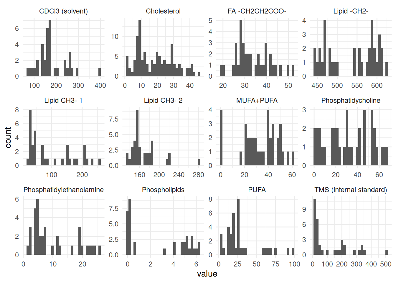
We want to keep it simple for now, as this workshop isn’t about making nice figures, it’s mainly about how to build reproducible pipelines. So for now, run styler with the Palette (Ctrl-Shift-PCtrl-Shift-P, then type “style file”), then run the pipeline with the Palette (Ctrl-Shift-PCtrl-Shift-P, then type “targets run”) to check that everything builds correctly. Open the updated HTML file to check how it looks. Then, we’ll add and commit the changes to the Git history with Ctrl-Alt-MCtrl-Alt-M or with the Palette (Ctrl-Shift-PCtrl-Shift-P, then type “commit”) and push the changes up to GitHub.
Time for you to convert the code into a function.
18.7 🧑💻 Exercise: Convert the plot code to a function
Note🧑🏫 Teacher note
After the exercise time has passed, ask how many have completed this exercise. Depending on how many have finished, help the ones who haven’t finished and tell those who have to move on to the next exercise.
Time: ~10 minutes.
For now, we will only take the code to make the distribution plot and convert it into a function. Just like you did with the create_table_descriptive_stats() function in the exercise above, complete these tasks, using the scaffolding code below to help you get started:
docs/learning.qmd
create_plot_distributions <- function(data) {
data |>
___
}
# Use it like, which should give the same output as before.
create_plot_distributions(lipidomics)Wrap the plot code inside
docs/learning.qmdwithfunction() {...}and name the new functioncreate_plot_distributions.Replace
lipidomicswithdataand putdataas an argument inside the brackets offunction()(already done in the scaffolding code).Add
ggplot2::to the start of each ggplot2 function used inside your function.Style using the Palette (Ctrl-Shift-PCtrl-Shift-P, then type “style file”) to make sure it is formatted correctly.
With the cursor inside the function, add some roxygen documentation with Ctrl-Shift-Alt-RCtrl-Shift-Alt-R or with the Palette (Ctrl-Shift-PCtrl-Shift-P, then type “roxygen comment”). Remove the lines that contain
@examplesand@export, then fill in the other details (like the@paramsandTitle). In the@returnsection, write “A plot object.”Cut and paste the function over into the
R/functions.Rfile.Source the
R/functions.Rfile with Ctrl-Shift-SCtrl-Shift-S or with the Palette (Ctrl-Shift-PCtrl-Shift-P, then type “source”) and then test the code by runningcreate_plot_distributions(lipidomics)in the Console. If it works, do the last task.Save both files and then open the Git interface and commit the changes you made to them with Ctrl-Alt-MCtrl-Alt-M or with the Palette (Ctrl-Shift-PCtrl-Shift-P, then type “commit”). Finally push your changes up to GitHub.
Click for the solution. Only click if you are struggling or are out of time.
## This should be in the R/functions.R file.
#' Plot for basic distribution of metabolite data.
#'
#' @param data The lipidomics dataset.
#'
#' @return A plot object.
#'
create_plot_distributions <- function(data) {
data |>
ggplot2::ggplot(ggplot2::aes(x = value)) +
ggplot2::geom_histogram() +
ggplot2::facet_wrap(ggplot2::vars(metabolite), scales = "free") +
ggplot2::theme_minimal()
}
# Testing the function
# create_plot_distributions(lipidomics)18.8 🧑💻 Exercise: Adding the plot function to the pipeline
Time: ~10 minutes.
Add the plot function you just created in the exercise above as a tar_target() item within the list() at the bottom of the _targets.R file and as an output in the docs/learning.qmd file.
Open the
_targets.Rfile and add a newtar_target()to the end of thelist(). Follow the same pattern as you’ve done with the other targets: Setnametoplot_distributionsandcommandtocreate_plot_distributions()withlipidomicsas the argument.Style the file using the Palette (Ctrl-Shift-PCtrl-Shift-P, then type “style file”).
Run
targets::tar_visnetwork()using the Palette (Ctrl-Shift-PCtrl-Shift-P, then type “targets visual”) and runtargets::tar_outdated()with the Palette (Ctrl-Shift-PCtrl-Shift-P, then type “targets outdated”) to see what has been changed.Run
targets::tar_make()using the Palette (Ctrl-Shift-PCtrl-Shift-P, then type “targets run”) to run the pipeline with the added target.Re-run
targets::tar_visnetwork()using the Palette (Ctrl-Shift-PCtrl-Shift-P, then type “targets visual”) to see the updated pipeline graph. You should see that the new item is now up to date.Open the
docs/learning.qmdfile and go to the bottom of the file. Create a new header called## Results: Distribution plotand add a new code chunk below it with Ctrl-Alt-ICtrl-Alt-I or with the Palette (Ctrl-Shift-PCtrl-Shift-P, then type “new chunk”). In this code chunk, usetar_read()to insert the output from theplot_distributionstarget and print it.Style the file using the Palette (Ctrl-Shift-PCtrl-Shift-P, then type “style file”).
Run
targets::tar_make()with the Palette (Ctrl-Shift-PCtrl-Shift-P, then type “targets run”) to build the pipeline again. Then runtargets::tar_visnetwork()using the Palette (Ctrl-Shift-PCtrl-Shift-P, then type “targets visual”) to see the updated pipeline graph.Open the updated HTML file to check out how it now looks.
If everything is good, then commit the changes to the Git history with Ctrl-Alt-MCtrl-Alt-M or with the Palette (Ctrl-Shift-PCtrl-Shift-P, then type “commit”). Then push your changes up to GitHub.
Click for the solution. Only click if you are struggling or are out of time.
_targets.R
list(
# ...,
tar_target(
name = plot_distributions,
command = create_plot_distributions(lipidomics)
)
)Click for the solution. Only click if you are struggling or are out of time.
docs/learning.qmd
tar_read(plot_distributions)
18.9 🧑💻 Extra exercise: Test out how tar_outdated() and tar_visnetwork() work
Time: ~10 minutes.
Make a change to one of your functions and test out how the tar_outdated() and tar_visnetwork() work.
Open up the
R/functions.Rfile and go to thecreate_table_descriptive_stats()function.Add median and interquartile range (IQR) to the
dplyr::summarise()function, by adding it to the end oflist(mean = mean, sd = sd), after the secondsd. Note, IQR should look likeiqr = IQRsince we want the output columns to have a lowercase for the column names.Do the same thing as we did for the
Mean (SD)column usingglue::glue()to create a new column calledMedian (IQR). You can do this by adding another line below theMeanSDcode in themutate().Rename the column in the
dplyr::select()function to be more human-readable, likeMedian IQR.Style using the Palette (Ctrl-Shift-PCtrl-Shift-P, then type “style file”).
Run
tar_outdated()andtar_visnetwork()in the Console (or by using the Command Palette Ctrl-Shift-PCtrl-Shift-P, then “targets outdated” or “targets visual”). What does it show?Run
tar_make()in the Console or with the Palette (Ctrl-Shift-PCtrl-Shift-P, then type “targets run”). Re-check for outdated targets and visualize the network again.Check the updated HTML file to confirm that the table has the added statistics, either by opening the HTML file in the browser or by re-rendering the Quarto document with Ctrl-Shift-KCtrl-Shift-K or with the Palette (Ctrl-Shift-PCtrl-Shift-P, then type “render”).
Click for a potential solution. Only click if you are struggling or are out of time.
create_table_descriptive_stats <- function(data) {
data |>
dplyr::group_by(metabolite) |>
dplyr::summarise(dplyr::across(
value,
list(
mean = mean,
sd = sd,
median = median,
iqr = IQR
)
)) |>
dplyr::mutate(dplyr::across(
tidyselect::where(is.numeric),
~ round(.x, digits = 1)
)) |>
dplyr::mutate(
MeanSD = glue::glue("{value_mean} ({value_sd})"),
MedianIQR = glue::glue("{value_median} ({value_iqr})")
) |>
dplyr::select(
Metabolite = metabolite,
`Mean SD` = MeanSD,
`Median IQR` = MedianIQR
)
}18.10 🧑💻 Extra exercise: Make the plot prettier
Time: ~10 minutes.
If you still have time, make your plot prettier, while testing out how the tar_outdated() and tar_visnetwork() work, and re-building the products, as you make changes.
Open up the
R/functions.Rfile and go to thecreate_plot_distributions()function.Change the theme to something else. You can see the different themes by typing
ggplot2::theme_in the Console and pressing Tab to see the options.Change the x- and y-axes labels to something more descriptive by using
ggplot2::labs().Add a figure caption to the plot by adding
#| fig-cap: "Your caption here"at the very top of the code chunk that has yourtar_read()plot code indocs/learning.qmd.Style using the Palette (Ctrl-Shift-PCtrl-Shift-P, then type “style file”).
Run
tar_outdated()andtar_visnetwork()in the Console (or by using the Command Palette Ctrl-Shift-PCtrl-Shift-P, then “targets outdated” or “targets visual”). What does it show?Run
tar_make()in the Console or with the Palette (Ctrl-Shift-PCtrl-Shift-P, then type “targets run”). Re-check for outdated targets and visualize the network again.Check the updated HTML file to confirm that the table has the added statistics, either by opening the HTML file in the browser or by re-rendering the Quarto document with Ctrl-Shift-KCtrl-Shift-K or with the Palette (Ctrl-Shift-PCtrl-Shift-P, then type “render”).
Click for a potential solution. Only click if you are struggling or are out of time.
# This has some potential changes.
create_plot_distributions <- function(data) {
data |>
ggplot2::ggplot(ggplot2::aes(x = value)) +
ggplot2::geom_histogram() +
ggplot2::facet_wrap(ggplot2::vars(metabolite), scales = "free") +
ggplot2::theme_classic() +
ggplot2::labs(
x = "Metabolite Value",
y = "Count"
)
}18.11 Summary
Build up targets piece by piece. Start at the end (e.g. the report) and work backwards. Let targets save the pipeline output and store the results for you, rather than keep them in your Git history.
Aim to have each target do one thing and to use one function per target. This keeps things a bit easier for you to track and manage, and keeps the pipeline smaller and more manageable.
Within R Markdown / Quarto files, use
targets::tar_read()to access saved pipeline outputs. To include the Quarto in the pipeline, use tarchetypes and the functiontar_quarto().
18.12 Survey
Please complete the survey for this session:
18.13 Code used in session
This lists some, but not all, of the code used in the section. Some code is incorporated into Markdown content, so is harder to automatically list here in a code chunk. The code below also includes the code from the exercises.
use_package("tarchetypes")
use_package("quarto")
use_git_ignore("_targets.yaml")
use_git_ignore("*_files")
use_git_ignore("*.html")
use_package("tidyverse", "depends")
lipidomics |>
  group_by(metabolite) |>
  summarise(across(value, list(mean = mean, sd = sd))) |>
  mutate(across(where(is.numeric), \(x) round(x, digits = 1))) |>
  mutate(MeanSD = glue::glue("{value_mean} ({value_sd})")) |>
  select(Metabolite = metabolite, "Mean SD" = MeanSD)
use_package("glue")
#' Calculate descriptive statistics of each metabolite.
#'
#' @param data The lipidomics dataset.
#'
#' @return A data.frame/tibble.
#'
create_table_descriptive_stats <- function(data) {
  data |>
    dplyr::group_by(metabolite) |>
    dplyr::summarise(dplyr::across(value, list(mean = mean, sd = sd))) |>
    dplyr::mutate(dplyr::across(
      tidyselect::where(is.numeric),
      \(x) round(x, digits = 1)
    )) |>
    dplyr::mutate(MeanSD = glue::glue("{value_mean} ({value_sd})")) |>
    dplyr::select(Metabolite = metabolite, `Mean SD` = MeanSD)
}

# create_table_descriptive_stats(lipidomics)

# Adding the new dependencies
# use_package("tidyselect")
list(
  ...,
  tar_target(
    name = table_descriptive_stats,
    command = create_table_descriptive_stats(lipidomics)
  )
)
tar_read(table_descriptive_stats) |>
  knitr::kable(
    caption = "The mean and standard deviation of metabolites in the lipidomics dataset."
  )
use_package("ggplot2")
ggplot(lipidomics, aes(x = value)) +
  geom_histogram() +
  facet_wrap(vars(metabolite), scales = "free") +
  theme_minimal()
## This should be in the R/functions.R file.
#' Plot for basic distribution of metabolite data.
#'
#' @param data The lipidomics dataset.
#'
#' @return A plot object.
#'
create_plot_distributions <- function(data) {
  data |>
    ggplot2::ggplot(ggplot2::aes(x = value)) +
    ggplot2::geom_histogram() +
    ggplot2::facet_wrap(ggplot2::vars(metabolite), scales = "free") +
    ggplot2::theme_minimal()
}

# Testing the function
# create_plot_distributions(lipidomics)
list(
  # ...,
  tar_target(
    name = plot_distributions,
    command = create_plot_distributions(lipidomics)
  )
)
tar_read(plot_distributions)
create_table_descriptive_stats <- function(data) {
  data |>
    dplyr::group_by(metabolite) |>
    dplyr::summarise(dplyr::across(
      value,
      list(
        mean = mean,
        sd = sd,
        median = median,
        iqr = IQR
      )
    )) |>
    dplyr::mutate(dplyr::across(
      tidyselect::where(is.numeric),
      ~ round(.x, digits = 1)
    )) |>
    dplyr::mutate(
      MeanSD = glue::glue("{value_mean} ({value_sd})"),
      MedianIQR = glue::glue("{value_median} ({value_iqr})")
    ) |>
    dplyr::select(
      Metabolite = metabolite,
      `Mean SD` = MeanSD,
      `Median IQR` = MedianIQR
    )
}
# This has some potential changes.
create_plot_distributions <- function(data) {
  data |>
    ggplot2::ggplot(ggplot2::aes(x = value)) +
    ggplot2::geom_histogram() +
    ggplot2::facet_wrap(ggplot2::vars(metabolite), scales = "free") +
    ggplot2::theme_classic() +
    ggplot2::labs(
        x = "Metabolite Value",
        y = "Count"
    )
}