Want to help out or contribute?

If you find any typos, errors, or places where the text may be improved, please let us know by providing feedback either in the feedback survey (given during class) or by using GitHub.

On GitHub open an issue or submit a pull request by clicking the " Edit this page" link at the side of this page.

9  Publicizing your analyses with a website

Disseminating our research and work is one of the key tasks of being a researcher. We researchers are sadly very limited in our focus on publishing papers, when our work can encompass much more than just papers and when there are other forms of publishing aside from papers. One of the most effective forms of disseminating content is in creating a website, thanks to the power of Google indexing.

With current software tools and services, Making simple websites like blogs has historically been fairly easy. Making websites presenting analytical work and outputs on the other hand, has been a difficult area. Over the last 10 years, many tools and packages have been created that try to simplify that task. They each have had their strengths, and their major flaws. The most recent software, though, is a massive improvement of previous attempts. In this session we will be covering how to make websites for code-based analysis projects that builds on top of R Markdown / Quarto that is familiar to many R users.

9.1 Learning objectives

The overall objective for this session is to:

1. Explain what a website is, what minimum files are needed, and how to use Quarto as a framework for creating them and including them as part of a pipeline.

More specific objectives are to:

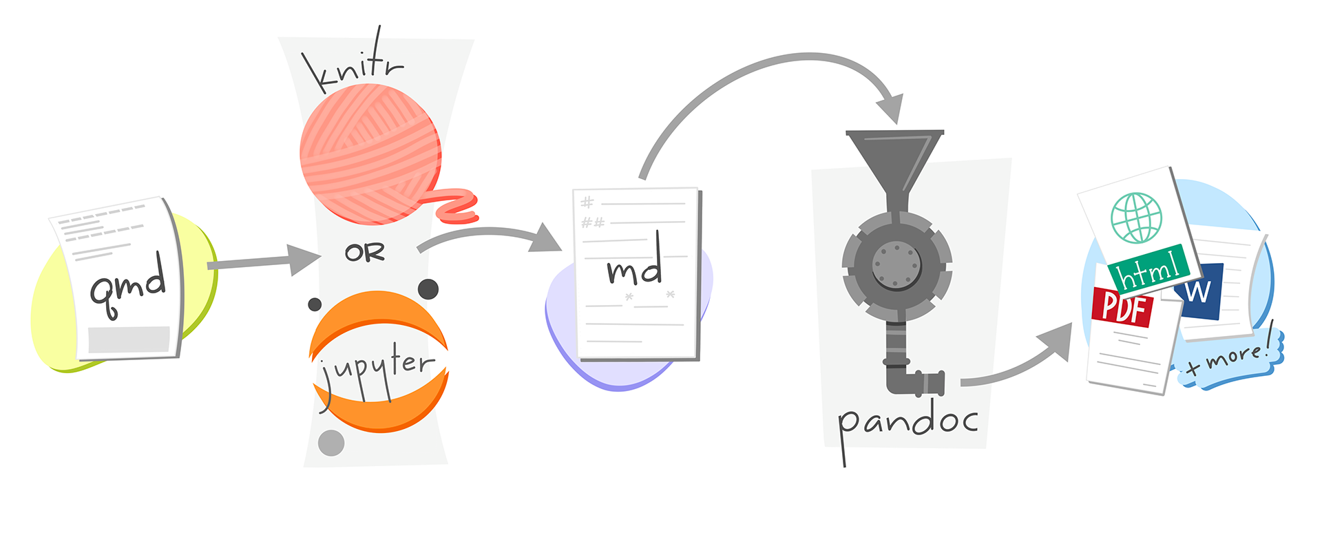
1. Describe how websites are essentially folders and files, where some files need to be named a specific way (like the index.html file).
2. Explain how Quarto executes R code in a document and creates different file formats from it, like Word or HTML. Use Quarto’s YAML header options, like format: docx or format: html, to create different file outputs.
3. Use the _quarto.yml file along with Quarto options to apply the understanding of how websites work and to build then them.
4. Use GitHub Actions to automate generating and uploading the website, then demonstrate how to make the material open by adding a license to the repository.
5. Continue applying the concepts and functions used from the previous sessions.

9.2 Websites, what they are and why researchers should create more

Reading task: ~3 minutes

Websites are a bit of a mystery in many ways. You open a browser, go to Google, search for something, click a link, scroll through the website, and read text, view images, or watch videos. But what are websites actually?

At their simplest and most basic core, a file on your computer and a webpage you click into are exactly the same. A website is literally a series of folders and files on a server in another country. Let’s use Posit (the new RStudio company name) as an example. The website https://posit.co/ is like a folder called posit.co/ on your computer. The website https://posit.co/resources/ (notice the resources/ ending) is like a resources/ folder in the posit.co/ main folder on your computer. But you might ask, you just said a webpage is like a file, so where is the file name in https://posit.co/resources/? Well, browsers do something special when they see an URL with no file ending: They assume some default files to look for. When a URL doesn’t include a file ending, the browser looks for files that are named either index or default. The most common file name for a webpage is index.html. But it can also be index.php, index.asp, or default.htm. We can test which file name a webpage is by typing the file name at the end of the URL. If we try https://posit.co/resources/index.html, we get a 404 error, meaning the file doesn’t exist. But if we try https://posit.co/resources/index.php, if works! So making a website is as simple as having HTML files in a folder and uploading that folder onto a website hosting service. The services themselves can be tricky to use, but some are dead easy, like GitHub Pages is, which we will show later on.

So why should researchers make websites? Because it is the easiest way to disseminate your work, your projects, who you are as a researcher, and to have more impact and outreach. Given the current tools available and their ease of use, there is no reason any researcher (even non-technical ones) couldn’t use websites as a way of publishing more of your work. Especially since if you are already learning about the workflow around using R, building functions, writing R Markdown (or Quarto), and using Git and GitHub, adding a website builder into this workflow is surprisingly easy.

Instructor note

Briefly go through this and reinforce that a website isn’t anything special, it’s only a different type of file then they typically use or create.

9.3 What is Quarto and why use it?

Reading task: ~5 minutes

Quarto is the next-generation R Markdown document generator. In terms of writing Markdown syntax, there is no difference between R Markdown and Quarto (since they both use Pandoc internally). The differences become obvious when you want to make more complex outputs like websites, books, or presentations or if you want to use another language like Python.

Quarto is “language-agnostic”, meaning it isn’t limited to only R (unlike R Markdown for the most part). And it is even easier to use than R Markdown and the documentation on Quarto’s website is very high quality. For instance, with the use of the “Search” feature in the Quarto website (in the right-hand corner), you can search the documentation very easily. Over the next few years, R Markdown will be slowly phased out in favour of Quarto, for good reason. It is an massive upgrade in features and usability.

Cartoon showing the general workflow that Quarto uses to create different file outputs. Artwork by @allison_horst.

Let’s start the comparison with the YAML header differences between R Markdown and Quarto:

Quarto: Word

format: docx

Quarto: HTML

format: html

R Markdown: Word

output: word_document

R Markdown: HTML

output: html_document

Another difference with Quarto compared to R Markdown is how code chunk options are set. While you can continue using knitr style code chunk options, it’s best to start switching to using the Quarto style. Compare them below.

knitr-style chunk options

```{r, warning=TRUE, message=TRUE}
1:5
```

#> [1] 1 2 3 4 5

Quarto-style chunk options

```{r}
#| warning: true
#| message: true
1:5
```

#> [1] 1 2 3 4 5

Why the change? They needed to develop an approach that worked with other languages as well, like Python. knitr is an R-specific package, so they needed a more language agnostic way of setting chunk options. A full list of the code chunk options is found in the Cell Reference section of the website.

As you can see, they aren’t too different. But as you use it more though, it becomes obvious how powerful Quarto is.

We can use the same keybinding shortcut as with R Markdown: with or with the Palette (, then type “render”). You can also use the Command Palette with followed by typing “render”.

One big upgrade from R Markdown is that Quarto has a strong focus on scholarly writing and formatting, for instance by adding authors and affiliation metadata that gets added to the output document. It looks like:

author:
  - name: Jane
    orcid: 0000-0000-0000-0000
    email: mymail@email.com
    affiliations:
      - name: Insitution Name
        address: Street 10
        city: City
        postal-code: 0000

9.4 Exercise: Add author information to the YAML in the Quarto file

Time: ~10 minutes.

In the doc/learning.qmd file, add your author information to the YAML header.

1. Add the author: metadata below the title: and above the format: metadata.
2. Include your name and affiliations (with only the - name: for institution).
3. Render the document with or with the Palette (, then type “render”). See what gets changed.
4. Replace format: html with format: docx and re-render the document. Switch back to html.
5. Commit the changes to the Git history with or with the Palette (, then type “commit”).

9.5 Using Quarto to build a project website

Now for the fun part, to use Quarto to build a website! At this stage, we only need two files: An index.qmd file and a _quarto.yml file. As we covered above, a browser will always look for a file called index when the URL is only a folder. So for our main project folder, we need this file. Let’s create this file with usethis to both create and than open it:

edit_file("index.qmd")

We won’t add much for now, only need to add a # header:

# Lipidomics study

Next, let’s create the _quarto.yml file that will have all the settings for the website.

edit_file("_quarto.yml")

There are many “top-level” settings that we can include in this file. The first one is the project: metadata, which tells Quarto details about the project as a whole. Since we want to create website, the option to set it would be type: website:

project:
  type: website

The next bit is to tell Quarto some details about the website. Websites in general are structured with the content, a navigation bar (“navbar”), and possibly some links on the side (think of how websites like YouTube or Twitter are structured). This is the same for Quarto. Each included .Rmd, .md, or .qmd files are the content and Quarto adds the navbar. But we have to include what gets added to the navbar.

The first “top-level” metadata is website: and the first second-level metadata is usually the title: of the website (that will be shown on the navbar). Next, let’s set up the navbar: second-level header. There are two sub-levels to navbar:, left: and right:. These tell Quarto what links should be put on the right-side of the navbar or the left-side. We’ll start with the left:. Underneath, we need to give it a list of either file names or a pair of href: and text: or icon: metadata. To keep things simple, we’ll use the href: and text: for each item for the index.qmd and the doc/learning.qmd files. Like a list in Markdown, a list in YAML starts with a -, where a pair of metadata belong to a single -. Our website: settings should look like this now:

website:
  title: "Lipidomics analysis"
  navbar:
    left:
      - href: index.qmd
        text: "Home"
      - href: doc/learning.qmd
        text: "Report"

After we’ve set the settings for the website:, we need to tell Quarto what output files to create. We could do this for each individual file, by adding format: html to each YAML header. But we’d be duplicating a lot of options and it would be annoying to change all of them if you wanted something different. Instead, we can put it in the _quarto.yml file and set the format: for all files in the project. Like the website: and project: settings, format: is a “top-level” option (meaning it doesn’t go under any other option in the file). There are many many options in format: we can set, but the biggest one is what theme: you want. There are several theme templates listed on the Quarto HTML Theming page. We’ll use a simple one called simplex.

Tip

You can always override the project-level settings from the _quarto.yml file by using the format: (or other options) in the YAML header of an individual Markdown file.

format:
  html:
    theme: simplex

Since we now have set the output format to HTML in the _quarto.yml file, let’s remove the same setting from the doc/learning.qmd file, so that both format: and (if it exists) execute: is removed.

While we have enough for Quarto to know how to build the website, let’s add one more thing to the Quarto settings. For documents on an analysis, we usually want to show the output of code but not the code itself. In knitr, there is a code chunk option echo that hides the code from the final output document. In Quarto, you can set project-level knitr options with the top-level metadata knitr: along with the second-level metadata opts_chunk:. Below it we can add settings that affect code chunks, like echo. Let’s hide all code from the website:

knitr:
  opts_chunk:
    echo: false

Tip

When building a website, Quarto will render all .md, .Rmd, and .qmd files in the project. To stop Quarto from rendering certain files, you can either prefix the file with _ (e.g. _learning.qmd) or you can use the render: setting and use ! before the file name you want to not render, which looks like this in the _quarto.yml file:

project:
  type: website
  render:
    - "!doc/learning.qmd"

Now let’s build the website. You can either use the “Render” button on the top or use for “Build”. Let’s do it now. The website should pop up in either the Viewer Pane or as a new window. If not, we can debug what’s going on.

The next step is to commit the changes we’ve made, but you’ll also see that a new folder called _site/ has been created. This folder contains all the files that form the website, like the HTML files and style files. While we could add these files to the Git history and make it so that GitHub uses those to host as a website, we’re going to set up GitHub later to build the website for us automatically. So we’ll add the _site/ folder to the .gitignore file with:

use_git_ignore("_site")

Now we can commit the changes to the _quarto.yml, the .gitignore file, and the index.qmd file to the Git history with or with the Palette (, then type “commit”).

9.6 Exercise: Add collaboration setting to _quarto.yml file and update targets

Time: ~5 minutes.

Like we did in Chapter 5 with the editor setting we added in our Quarto file, let’s make this setting global to the whole project. Cut and paste that metadata from doc/learning.qmd into the bottom of _quarto.yml:

editor:
  markdown:
    wrap: 72
    canonical: true

Next, update the _targets.R file by changing:

• the name argument to quarto_website, since we’re building a site now not just docs, and,
• the path argument to point to the main project folder "." (. means “the same folder _targets.R is in)

It should look like this now:

tar_quarto(
  name = quarto_website,
  path = "."
)

Then, finish up by:

1. Running targets::tar_make() with the Palette (, then type “targets run”) to rebuild everything and test that the pipeline works.
2. Commit your changes to the Git history with or with the Palette (, then type “commit”).

9.7 Automate rendering the website

There is a way that we could create the website and save it in the _site/ folder, commit it to Git, and have GitHub host the website for us. But than we’d be saving a lot of files that would need to be updated quite often, which is annoying to keep track of. Instead, we can make use of GitHub Actions to build and publish our website for us, including rendering all the R code.

There is a way to have GitHub completely (re-)build the website from scratch each time, including running any R code. However, our project doesn’t have much R code and we have data that we don’t keep in the project Git history. So we need to run the computations locally first so GitHub and build the website without the data. This is done through something called “execution freezes”. In the _quarto.yml file, add this metadata settings to the bottom:

execute:
  freeze: auto

Then when we re-render the website with , there will be a new folder created called _freeze/. Inside this folder are instructions to Quarto on how to run the code chunks inside the .qmd file. Commit this folder to the Git history with or with the Palette (, then type “commit”).

To get GitHub Actions to build the website we need to do two things first. Run a command to set things up and then add a new Action workflow file.

To set our repository up for the Action, we need to run quarto publish gh-pages once in the Terminal (not the R Console). We open the Terminal either through the menu Tools -> Terminal -> New Terminal or with the Command Palette () along with typing the text “terminal”.

quarto publish gh-pages

Or, we can make use of the R’s system() function by typing in the R Console:

system("quarto publish gh-pages")

Next is add the Action workflow file:

edit_file(".github/workflows/build-website.yaml")

Then we can copy and paste the template code from the Quarto Example Action file, which is (slightly modified) below. We don’t need to understand this code, at least not for this course. Because it is template code, it’s there to be copied and pasted (for the most part).

on:
  push:
    branches: 
      - main
      - master

name: Render and Publish

permissions:
  contents: write
  pages: write

jobs:
  build-deploy:
    runs-on: ubuntu-latest
    steps:
      - name: Check out repository
        uses: actions/checkout@v4
        
      - name: Set up Quarto
        uses: quarto-dev/quarto-actions/setup@v2
        with:
          # To install LaTeX to build PDF book 
          tinytex: false
          # uncomment below and fill to pin a version
          # version: 0.9.600
          
      # From https://github.com/r-lib/actions/tree/v2-branch/setup-r
      - name: Publish to GitHub Pages (and render)
        uses: quarto-dev/quarto-actions/publish@v2
        with:
          target: gh-pages
        env:
          # this secret is always available for github actions
          GITHUB_TOKEN: ${{ secrets.GITHUB_TOKEN }} 

Let’s commit this new file to the Git history with or with the Palette (, then type “commit”) and push the changes up to GitHub. While we wait for the GitHub Action to finish, complete the next exercise.

9.8 Exercise: Add licensing information to repository

Time: ~10 minutes.

You’ve now created and published a website! If you value sharing though, there’s a few extra things you need to do. Whenever you create something, legally it is copyrighted to you. If you do nothing else, no one is able to use what you share because legally they are not allowed to. That’s where licenses come in. A license is a legal document that tells others what they can and can’t do with your copyrighted material. If you are publishing research work or other creative works and you want others to easily re-use it, you need to add a license document to your repository. A commonly used and recommended license for research and creative work is the Creative Commons Attribution 4.0 license, so we will use that.

1. In the R Console, type out use_ccby_license().

2. Add a simple license text to the bottom of each webpage by opening _quarto.yml, going to the website: section, and adding this to the bottom of it, so it should look like this:

   website:
     title: "Lipidomics analysis"
     navbar:
       left:
         - href: index.qmd
           text: "Home"
         - href: doc/learning.qmd
           text: "Report"
     page-footer:
       center:
         - text: "License: CC BY 4.0"

3. Check that it works by rendering the website locally again with . Scroll to the bottom of the webpage that pops up to check that it has been added.

4. If it shows up, commit the changes to the Git history with or with the Palette (, then type “commit”) and then push up to GitHub. Wait for the GitHub Action to complete and you can now check that your website online also has the changes.

Next, let’s add some discoverability items to the README.md file and to the GitHub repository.

1. Go to your project’s GitHub repository. A quick way of doing that is using browse_project() from usethis.

2. Confirm that the Actions worked by going to the “Actions” tab. If there is a green check mark there, than continue to the next item. Otherwise, put up a “help sticky”.

3. On your project’s GitHub repository and go to Settings -> Pages. You should see a link to your new website. Copy that link.

4. Go to the “Code” tab, then click the gear icon on the right side, to the right of “About”. In the box that pops up, paste the link in the “Website” textbox.

5. In your RStudio project, open up the README.md file (e.g. with edit_file("README.md")). Add some text below the first # header, pasting the link where the LINK text is in this template:

   Check out the project's [website](LINK).

6. Commit the changes to the README.md to the Git history with or with the Palette (, then type “commit”).

Tip

Sometimes you might make a change to files that aren’t part of the website and don’t want to trigger the GitHub Action, since it would be a waste of resources (computing time still costs energy). GitHub Actions run every time you push up. So if you don’t want the last commit in the Git history to trigger the Actions, you can add the text [skip actions] to the end of the commit message.

9.9 Summary

• Use Quarto, along with their referring to their documentation, to create various types of output documents, including websites.
• Add an index.qmd file as well as the _quarto.yml file with Quarto settings to build a website.
• Make use of execution freezes and GitHub Actions to host your website on GitHub.
• Add a license file (for instance, with use_ccby_license()) to allow others to re-use your work.